CyteArc’s memory limits do not prevent you from using an external analysis method. You can read its neighborhood graphs, process count blocks, and add cell-level results through public APIs. When another tool needs its own data format, export the cells and genes that method requires.
This tutorial calculates a graph statistic, streams counts without loading the complete matrix, creates a custom cell selection, and exports that selection to AnnData or a separate CyteArc store.
Import an existing store
The prepared PBMC store supplies counts and a saved example run labeled docs_default.
Open the downloaded store directly because the examples write custom artifacts and metadata, then
reuse the run’s frozen selection, graph, feature selection, and UMAP. The prepared store’s active
I matches the run’s analysis selection.
See Build a neighborhood graph stage by stage to build a graph by hand.
# Calculate custom statistics from graph weights and count blocks.
import numpy as np

import cytearc

# Keep routine progress messages out of the teaching output.
cytearc.configure_output(level="WARNING", progress=False)

# Download the prepared example, including its saved analysis.
dataset = cytearc.cytebase.connect("cytearc_docs").download_dataset(
    "tenx_5K_pbmc_rnaseq", destination="cytearc_datasets", zarr=True
)
Started: 2026-10-11T18:54:43.100120Z | Wall time: 3.037 s
Open the downloaded store and its saved analysis.
# Open the datastore for the following analysis.
ds = cytearc.DataStore(f"{dataset}/data.zarr", nthreads=4)

# Open the saved analysis and retain its exact results.
run = ds.pipeline.open(label="docs_default")

# Keep the reference to the saved connectivity graph.
graph_ref = run["connectivity_map"]

# Inspect the opened assays and their dimensions.
ds
DataStore has 3948 (5025) cells with 1 assays: RNA
Cell metadata:
'I', 'ids', 'names', 'RNA_G2M_score', 'RNA_S_score',
'RNA_UMAP1', 'RNA_UMAP2', 'RNA_cell_cycle_phase', 'RNA_clusters', 'RNA_doublet_score',
'RNA_leiden_cluster', 'RNA_nCounts', 'RNA_nFeatures', 'RNA_paris_cluster', 'RNA_percentMito',
'RNA_percentRibo'
RNA assay has 33538 features and following metadata:
'I', 'ids', 'names', 'dropOuts', 'feature_type',
'genome', 'nCells'Started: 2026-10-11T18:54:46.139489Z | Wall time: 5.169 s
Calculate from the graph
Suppose an external method needs a measure of how strongly each cell connects to its neighbors.
graph.load returns the selected neighborhood graph as a SciPy CSR matrix. Summing each row
gives that cell’s total edge weight in the symmetric graph: cells with larger sums have stronger
weighted connections in this particular graph. This is a graph statistic, not a biological
confidence score or an automatic quality-control rule.
# Load the symmetric connectivity graph as a sparse matrix.
graph = ds.graph.load(graph=graph_ref, symmetric=True, upper_only=False)

# Sum the edge weights connected to each cell.
graph_strength = np.asarray(graph.sum(axis=1)).ravel()

# Save the values in cell metadata using the stated selection.
ds.cells.insert(
    column_name="customGraphStrength", values=graph_strength, key="I", overwrite=True
)

# Summarize the graph size and the new per-cell connectivity statistic.
{
    "cells": int(graph.shape[0]),
    "edges": int(graph.nnz),
    "customGraphStrength mean": float(graph_strength.mean()),
}
{'cells': 3948, 'edges': 64990, 'customGraphStrength mean': 8.832276344299316}Started: 2026-10-11T18:54:51.310527Z | Wall time: 0.117 s
The insert writes one value per active cell in graph row order. The summary shows the graph size and the mean of the new column.
# Locate high and low graph connectivity on the saved embedding.
ds.plots.embedding(layout=run["umap"], color_by="customGraphStrength")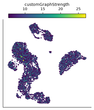
Started: 2026-10-11T18:54:51.429243Z | Wall time: 1.097 s
The plot asks where cells have stronger or weaker weighted connectivity in this specific graph. Rebuilds with another feature set or neighbour count need a new statistic.
Stream count blocks
A custom calculation can stay within a small memory budget by processing one count block at a
time. Avoid .compute() on a matrix that may exceed memory. Select the frozen run’s cells and
highly variable genes before streaming, then keep only the small per-cell results from each block.
Here we count detected HVGs per active cell:
# Locate the run's cells on the stored count-matrix axis.
cell_index = np.flatnonzero(run.cells.fetch_all("I"))

# Read the run's highly variable gene selection.
hvg_values = np.asarray(run.features.fetch_all("highly_variable_features"), dtype=bool)

# Locate those genes on the stored feature axis.
feature_index = np.flatnonzero(hvg_values)

# Create a lazy view of the selected cells and genes.
selected_counts = ds.RNA.rawData[:, feature_index][cell_index, :]

# Check the selected matrix dimensions before streaming counts.
{"selected cells": len(cell_index), "selected genes": len(feature_index)}
{'selected cells': 3948, 'selected genes': 500}Started: 2026-10-11T18:54:52.528527Z | Wall time: 0.269 s
Count detected genes one block at a time.
# Collect one small vector of detection counts per block.
detected_blocks = []

# Process a bounded count block without loading the full matrix.
for count_block in selected_counts.stream_blocks(
    nthreads=4, msg="Calculating custom detection statistic"
):

    # Keep this result in its original processing order.
    detected_blocks.append(np.count_nonzero(count_block, axis=1))

# Check how many cell results were collected across the blocks.
sum(len(block) for block in detected_blocks)3948Started: 2026-10-11T18:54:52.799586Z | Wall time: 0.455 s
Collect the per-cell results and save them in metadata.
# Join the block results in their original cell order.
detected_hvgs = np.concatenate(detected_blocks)

# Save the values in cell metadata using the stated selection.
ds.cells.insert(
    column_name="customDetectedHVGs", values=detected_hvgs, key="I", overwrite=True
)

# Summarize the per-cell detected-gene counts.
{
    "cells": int(detected_hvgs.size),
    "customDetectedHVGs mean": float(detected_hvgs.mean()),
    "customDetectedHVGs max": int(detected_hvgs.max()),
}
{'cells': 3948,
'customDetectedHVGs mean': 123.48024316109422,
'customDetectedHVGs max': 250}Started: 2026-10-11T18:54:53.256759Z | Wall time: 0.029 s
stream_blocks preserves row order. Because active I is the frozen run selection, inserting with
that key keeps each streamed value aligned with its metadata row.
The summary checks that every streamed cell received a detection count.
Create custom selections
A Boolean cell column can become a cell_key. Selecting cells this way does not delete their
counts: the selection controls which rows an operation reads, while the original store remains
available for a different selection later.
Use fill_value=False when the new key is defined only for currently active cells: the inactive
cells then hold False. Without it they are recorded as missing, which a key never selects either.
Here we keep cells above the lowest quarter of graph strength as an example of making a selection.
This is an illustration of the API, not a recommended quality-control filter:
# Keep cells above the lowest quarter of graph strength.
well_connected = graph_strength >= np.quantile(graph_strength, 0.25)

# Save the values in cell metadata using the stated selection.
ds.cells.insert(
    column_name="wellConnected",
    values=well_connected,
    fill_value=False,
    key="I",
    overwrite=True,
)

# Check how many active cells pass the custom selection.
{"selected cells": int(well_connected.sum()), "active cells": len(well_connected)}
{'selected cells': 2961, 'active cells': 3948}Started: 2026-10-11T18:54:53.287760Z | Wall time: 0.019 s
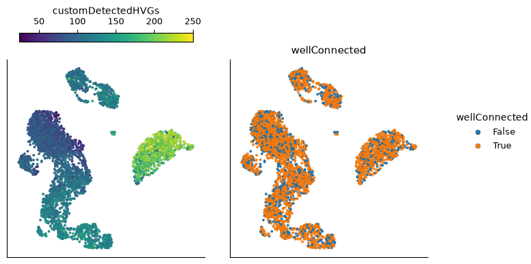
# Compare detected-gene counts and the custom cell selection.
ds.plots.embedding(
    layout=run["umap"], color_by=["customDetectedHVGs", "wellConnected"], n_columns=2
)
Started: 2026-10-11T18:54:53.309141Z | Wall time: 0.529 s
The first panel checks where the streamed count statistic varies. The second shows the lower-quartile graph-strength exclusion created from the same active cell order.
Pass a small selection to another tool
To pass a selection to a tool such as Scanpy, use to_anndata. It creates an in-memory AnnData
object, so select the cells and genes you need before materializing it. Here we export the custom
cell selection and a six-gene marker panel:
# Choose a small marker panel for the comparison.
panel_genes = ["CD3D", "MS4A1", "CD14", "LYZ", "NKG7", "GNLY"]

# Materialize only the selected cells and marker panel.
adata = ds.to_anndata(cell_key="wellConnected", feature_names=panel_genes)

# Check the exported dimensions and feature identifiers.
adata.shape, adata.var_names.tolist()
((2961, 6),
['ENSG00000167286',
'ENSG00000156738',
'ENSG00000170458',
'ENSG00000090382',
'ENSG00000105374',
'ENSG00000115523'])Started: 2026-10-11T18:54:53.841484Z | Wall time: 1.130 s
to_anndata drops unselected features.
It indexes var by gene ids (Ensembl here); gene symbols stay in var["names"].
So adata.var_names after feature_names=panel_genes lists ids, not the panel symbols.
Check adata.var["names"] when you need the symbols.
Omit feature_names to include every feature, provided the resulting AnnData fits in memory.
See Import and export for H5AD and Matrix Market export, and Explore a remote dataset when
the count source itself must remain remote.
Write a selected CyteArc store
Use SubsetZarr when the next analysis should stay in CyteArc. It writes only the selected cells
while retaining every feature in the listed assays. This differs from the six-gene AnnData above:
the resulting store can support analyses using a new feature set.
# Create a temporary destination separate from the source store.
from pathlib import Path
from tempfile import TemporaryDirectory

export_directory = TemporaryDirectory()
subset_path = Path(export_directory.name) / "well_connected.zarr"

# Copy the chosen cells with all RNA genes and their existing filter flags.
writer = cytearc.SubsetZarr(
    zarr_loc=str(subset_path),
    assays=[ds.RNA],
    cell_key="wellConnected",
    reset_cell_filter=False,
)
writer.dump()

# Confirm the cell and gene counts in the independent subset.
subset = cytearc.DataStore(str(subset_path))
{"exported cells": subset.cells.N, "retained genes": subset.RNA.feats.N}
{'exported cells': 2961, 'retained genes': 33538}Started: 2026-10-11T18:54:54.975546Z | Wall time: 2.732 s
Choose a persistent destination instead of TemporaryDirectory when you want to keep the subset
after the notebook session.
Extension boundary
Direct arbitrary artifact writing is not a stable public extension API.
Do not mutate ds.z, ds.zw, _matrix_z, or other private storage attributes from analysis code.
Those objects expose implementation layout and can change as CyteArc changes.
Use public metadata insertion, result-returning methods, graph loading, block streams, and export APIs. Pipeline callbacks provide read-only execution events; their contract is documented in Analysis pipeline API reference.