Explore CyteBase

CyteBase provides cloud-hosted CyteArc DataStores that you can connect to directly for exploration and analysis, without first downloading an H5AD or a complete data.zarr. Search the catalog, choose a dataset, and open its published store from a local notebook or a Python session on cloud compute.

CyteArc reads metadata and count blocks over the network as needed. Computation runs where your Python session runs; connecting to CyteBase does not provision a cloud worker. Shared stores are read-only. A mount lets you save new analysis results on your execution machine while the counts stay in CyteBase.

This tutorial uses datasets sourced from CELLxGENE. It searches the catalog, reads cell annotations, and plots the UMAP coordinates supplied by CELLxGENE. Gene expression comes from the published RNA counts; no new embedding or analysis pipeline is run in this walkthrough.

The saved results on this page were built with the CyteBase October 2026 release (2610), published in the public Nygen/cytebase-2610 bucket, which readers can access without credentials. Each release has its own bucket, so rerunning this page against 2610 reads the same catalog; cytebase.releases() lists newer releases.

Use the page download menu to save the source notebook. For a longer worked example, see the CyteBase case study: COVID-19 blood case study.

Install CyteArc’s SDK and plotting dependencies in your notebook environment:

# Install the CyteBase connector and a notebook environment.
uv pip install --prerelease allow 'cytearc[cytebase]' jupyterlab

When working from a CyteArc checkout, use uv sync --extra cytebase --extra extra and select its Python kernel. cytebase.Catalog() connects to the latest public release by default; this page pins version="2610". To use another bucket, pass bucket= to Catalog instead of version=, or omit both and set CYTEBASE_BUCKET before starting Jupyter. Explicit arguments take precedence over the environment variable. For a private bucket, supply HF_TOKEN through your environment or use your existing Hugging Face login. Keep credentials and private bucket names out of notebook source and outputs.

Connect and search¶

# Import the catalog client and notebook display tools.
import logging
from IPython.display import Markdown, display

import cytearc
from cytearc import cytebase

# Keep routine progress messages out of the teaching output.
cytearc.configure_output(level="WARNING", progress=False)

# HF retry messages include private bucket URLs; keep them out of shared outputs.
logging.getLogger("huggingface_hub").setLevel(logging.ERROR)

# Connect to the October 2026 release used for this page's saved results.
catalog = cytebase.Catalog(version="2610")

Started: 2026-10-12T13:54:14.773091Z | Wall time: 2.715 s

Catalog(version="2610") connects to the October 2026 release and keeps a small local copy of its catalog. Searches use this catalog, so they do not read any count data. By default, they return datasets ready to open.

The example is a single-nucleus RNA-seq dataset of human kidney cortex from donors with and without diabetic kidney disease (Wilson et al., 2022). Search for its author and tissue, then keep the returned identifier rather than constructing an ID yourself.

# Search the catalog for the dataset used in this example.
matches = catalog.search("wilson kidney cortex")

# Stop if the expected kidney dataset is not available.
if not matches:
    raise RuntimeError("The example kidney dataset is not ready in this bucket")

# Summarize dataset titles and sizes while keeping full IDs in the result rows.
match_preview = matches.to_markdown(
    columns=["cytebase_id", "title", "cell_count"], max_cell_chars=32
)

# Display the search summary before choosing a dataset.
display(Markdown(match_preview))

Started: 2026-10-12T13:54:17.490114Z | Wall time: 2.306 s

# Keep the dataset identifier returned by the catalog.
dataset_id = matches[0]["cytebase_id"]

# Read the dataset's scientific metadata and citation.
entry = catalog.dataset(dataset_id)

# Inspect the dataset record and source citation.
entry

Started: 2026-10-12T13:54:19.798251Z | Wall time: 4.555 s

entry is a DatasetEntry containing metadata about the scientific dataset. Displaying it reads the catalog and dataset record. It does not open the remote Zarr hierarchy. The citation and CELLxGENE links identify the original study; retain these when using the data.

Open the remote DataStore¶

catalog.open_datastore(entry.id) validates the published dataset version and build receipt, then returns a DataStore with zarr_mode="r". Counts remain remote and the SDK does not write back to the bucket. Keep this object as ds for metadata queries, plotting, and other datastore operations.

# Open the datastore for the following analysis.
ds = catalog.open_datastore(entry.id)

# Inspect the store's assays and dimensions.
ds

DataStore has 39176 (39176) cells with 1 assays: RNA
   Cell metadata:
            'I', 'ids', 'names', 'RNA_nCounts', 'RNA_nFeatures', 
            'RNA_percentMito', 'RNA_percentRibo', 'assay', 'assay_ontology_term_id', 'author_cell_type', 
            'cell_type', 'cell_type_ontology_term_id', 'development_stage', 'development_stage_ontology_term_id', 'disease', 
            'disease_ontology_term_id', 'donor_id', 'doublet_id', 'is_primary_data', 'library_uuid', 
            'mapped_reference_annotation', 'nCount_RNA', 'nCount_SCT', 'nFeature_RNA', 'nFeature_SCT', 
            'observation_joinid', 'percent.mt', 'percent.rpl', 'percent.rps', 'reported_diseases', 
            'sample_preservation_method', 'sample_uuid', 'self_reported_ethnicity', 'self_reported_ethnicity_ontology_term_id', 'seurat_clusters', 
            'sex', 'sex_ontology_term_id', 'suspension_type', 'suspension_uuid', 'tissue', 
            'tissue_ontology_term_id', 'tissue_type'
   RNA assay has 35469 features and following metadata:
            'I', 'ids', 'names', 'dropOuts', 'feature_biotype', 
            'feature_length', 'feature_reference', 'feature_type', 'nCells'

Started: 2026-10-12T13:54:24.354425Z | Wall time: 23.616 s

Small Zarr metadata objects are cached in memory for this open store. Count chunks are fetched when needed; the SDK does not maintain a persistent local count cache. Opening and plotting still depend on network latency.

The source H5AD may contain more embeddings than the pipeline imported. Check the imported keys before plotting:

# List the embeddings recorded in the source dataset.
print("Source embedding keys:", entry.source_embeddings())

# List the embeddings actually imported into the CyteArc store.
print("Imported embedding keys:", sorted(cytebase.embeddings(ds)))

# Select the imported UMAP without recomputing its coordinates.
umap_ref = cytebase.embedding(ds, "X_umap")

Source embedding keys: ['X_harmony', 'X_pca', 'X_umap']

Imported embedding keys: ['X_umap']

Started: 2026-10-12T13:54:47.971824Z | Wall time: 3.872 s

The current pipeline imports obsm/X_umap. An X_pca key in the source list alone does not mean its coordinates are available in the CyteArc store.

Read cell metadata¶

CELLxGENE annotations are stored beside CyteArc’s QC columns, such as RNA_nCounts and RNA_nFeatures. Request only the columns needed for a figure:

# Use pandas to inspect the cell annotations as a table.
import pandas as pd

# Choose the metadata fields needed for exploration.
wanted = ["cell_type", "tissue", "disease", "donor_id", "sex", "assay"]

# Keep only metadata fields available in this store.
columns = [column for column in wanted if column in ds.cells.columns]

# Read cell metadata and index it by cell ID.
meta = ds.cells.to_pandas_dataframe(["ids", *columns], key="I").set_index("ids")

# Preview cell types and donor groups without truncating annotation names.
with pd.option_context("display.max_colwidth", None):
    display(meta[["cell_type", "disease", "donor_id"]].head())

	cell_type	disease	donor_id
ids
AAACCTGAGTGTTAGA-1	epithelial cell of proximal tubule	normal	control_1
AAACCTGCAAGCGCTC-1	kidney loop of Henle thick ascending limb epithelial cell	normal	control_1
AAACCTGCACCAGATT-1	kidney loop of Henle thick ascending limb epithelial cell	normal	control_1
AAACCTGCAGTCAGAG-1	epithelial cell of proximal tubule	normal	control_1
AAACCTGCATGGAATA-1	kidney distal convoluted tubule epithelial cell	normal	control_1

Started: 2026-10-12T13:54:51.845275Z | Wall time: 10.092 s

This materializes the selected metadata columns as a pandas DataFrame, not the expression matrix. On a large atlas, metadata and coordinates still require memory proportional to the selected cells.

Use ds.cells.columns to check the available names. CyteArc replaces / and \ in imported column names with _ so they can be stored safely.

# Count cells assigned to each published cell type.
meta["cell_type"].value_counts().rename("cells").to_frame()

	cells
cell_type
epithelial cell of proximal tubule	11478
kidney distal convoluted tubule epithelial cell	8469
kidney loop of Henle thick ascending limb epithelial cell	7749
renal principal cell	3295
renal alpha-intercalated cell	2029
endothelial cell	1702
parietal epithelial cell	1103
podocyte	1069
kidney loop of Henle thin ascending limb epithelial cell	679
renal beta-intercalated cell	670
mesangial cell	385
fibroblast	338
leukocyte	210

Started: 2026-10-12T13:55:01.938620Z | Wall time: 0.009 s

Compare cell-type composition between the donor groups:

# Compare the cell counts or fractions across the selected groups.
pd.crosstab(meta["cell_type"], meta["disease"])

disease	normal	type 2 diabetes mellitus
cell_type
endothelial cell	1167	535
epithelial cell of proximal tubule	8818	2660
fibroblast	210	128
kidney distal convoluted tubule epithelial cell	6099	2370
kidney loop of Henle thick ascending limb epithelial cell	5432	2317
kidney loop of Henle thin ascending limb epithelial cell	324	355
leukocyte	54	156
mesangial cell	268	117
parietal epithelial cell	696	407
podocyte	679	390
renal alpha-intercalated cell	1491	538
renal beta-intercalated cell	376	294
renal principal cell	2053	1242

Started: 2026-10-12T13:55:01.949401Z | Wall time: 0.026 s

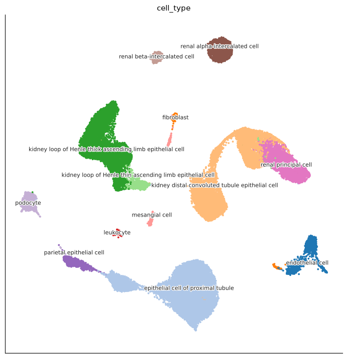
Plot the stored UMAP¶

ds.plots.embedding(layout=umap_ref, ...) uses the exact imported coordinates without recomputing UMAP. With a moderate number of cell types, the default legend placement writes each label on its cluster. A large atlas with many labels is better viewed with selected groups or legend_loc="none".

# Plot the published cell types and retain the figure for export.
cell_type_plot = ds.plots.embedding(
    layout=umap_ref, color_by="cell_type", figsize=(10, 7)
)

Published kidney UMAP colored and labeled by cell type, including tubular epithelial cells, intercalated cells, podocytes, endothelial cells, fibroblasts, and leukocytes.

Started: 2026-10-12T13:55:01.976529Z | Wall time: 11.770 s

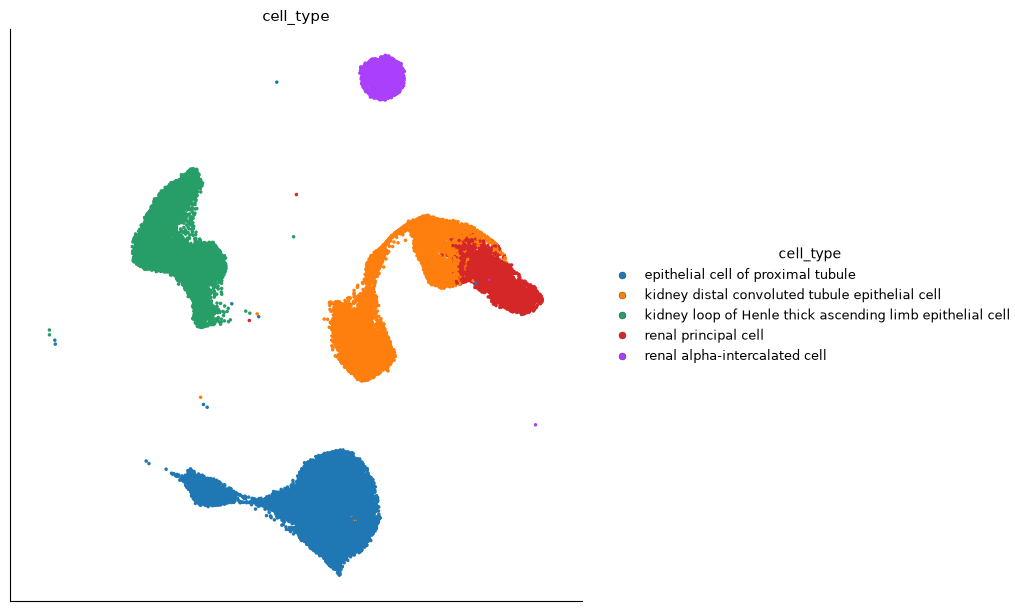
Focus on the five most common cell types without changing the source dataset:

# Select the five most common cell types for a closer view.
top_types = meta["cell_type"].value_counts().head(5).index.tolist()

# Focus the UMAP on the five most abundant cell types.
ds.plots.embedding(
    layout=umap_ref,
    color_by="cell_type",
    groups=top_types,
    figsize=(10, 6),
)

The published kidney UMAP restricted to its five most abundant cell types. Colors distinguish proximal tubule, distal convoluted tubule, thick ascending limb, principal, and alpha-intercalated cells.

Started: 2026-10-12T13:55:13.748015Z | Wall time: 8.485 s

Gene expression¶

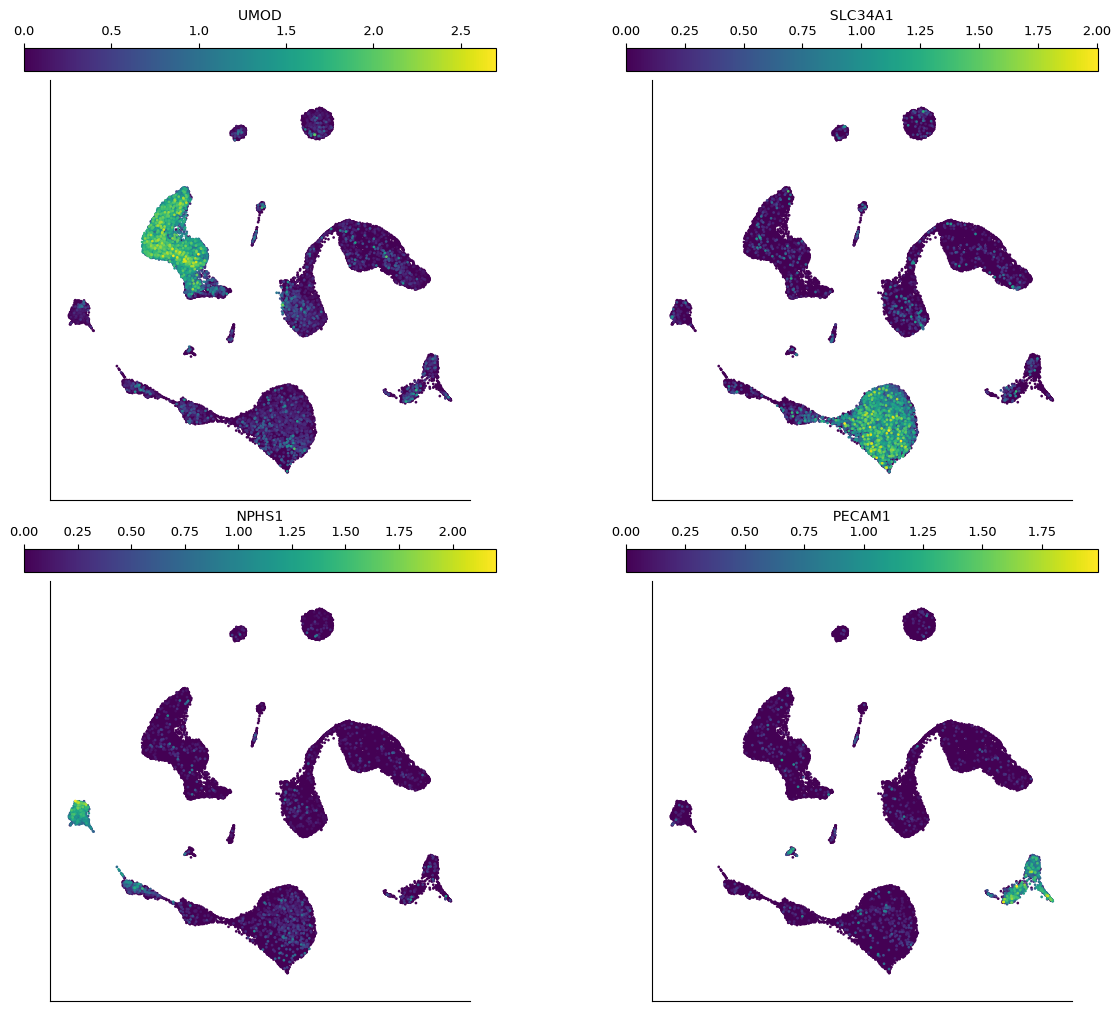
CyteArc looks up gene symbols without regard to case. Here we use UMOD for the thick ascending limb of the loop of Henle, SLC34A1 for the proximal tubule, NPHS1 for podocytes, and PECAM1 for endothelial cells. An unknown or ambiguous name raises an error, so check the feature metadata when adapting this panel to another dataset.

# Choose representative markers for the kidney populations.
genes = ["UMOD", "SLC34A1", "NPHS1", "PECAM1"]

Started: 2026-10-12T13:55:22.234517Z | Wall time: 0.003 s

Expression values are normalized on read; this example explicitly requests a log1p transform. Neither the count matrix nor the imported coordinates are modified. Drawing high values last makes expressing cells easier to see. Each gene is read from the remote counts, so every panel adds network reads.

# Specify how counts are normalized for the expression plots.
from cytearc.plotting import NormalizationSpec

# Plot the four kidney markers using log-normalized expression.
ds.plots.embedding(
    layout=umap_ref,
    color_by=genes,
    normalization=NormalizationSpec(transform="log1p"),
    sort_values=True,
    n_columns=2,
    figsize=(12, 10),
)

Kidney UMAP panels show log-normalized UMOD, SLC34A1, NPHS1, and PECAM1 expression in distinct regions corresponding to the selected marker populations.

Started: 2026-10-12T13:55:22.238621Z | Wall time: 22.918 s

Other plots from the same assay¶

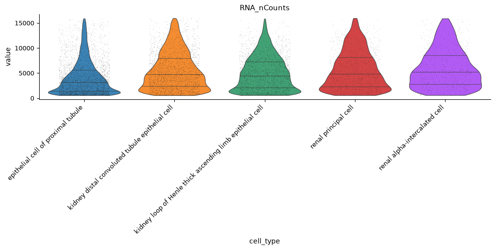
The read-only DataStore also supports plots from existing metadata and counts. For example, compare a QC measure across cell types:

# Select cell metadata fields for the comparison plots.
from cytearc.plotting import CellField

# Compare distributions within the stated groups.
ds.plots.distribution(
    "RNA_nCounts",
    grouping=CellField("cell_type"),
    groups=top_types,
    figsize=(10, 5),
)

Violin plots of total RNA counts across the five most common kidney cell types. Each distribution shows per-cell counts rather than a comparison of gene expression.

Started: 2026-10-12T13:55:45.158439Z | Wall time: 2.369 s

Gene distributions use the same interface; this optional example reads additional expression values:

# Compare distributions within the stated groups.
ds.plots.distribution(
    genes[:2],
    grouping=CellField("cell_type"),
    groups=top_types,
    figsize=(12, 5),
)

Coordinates for custom plots¶

Coordinates follow the embedding artifact’s frozen cell selection and are indexed by cell ID. Join on those IDs instead of assuming the same row order as a separate metadata table:

# Read coordinates indexed by the embedding's cell IDs.
coords = cytebase.embedding_coordinates(ds, umap_ref)

# Align metadata and coordinates by cell ID.
frame = coords.join(meta)

# Preview joined coordinates and full cell-type names in the same rows.
with pd.option_context("display.max_colwidth", None):
    display(frame[["umap_1", "umap_2", "cell_type"]].head())

	umap_1	umap_2	cell_type
ids
AAACCTGAGTGTTAGA-1	-0.523972	-8.470732	epithelial cell of proximal tubule
AAACCTGCAAGCGCTC-1	-7.073731	3.068685	kidney loop of Henle thick ascending limb epithelial cell
AAACCTGCACCAGATT-1	-6.279858	4.984632	kidney loop of Henle thick ascending limb epithelial cell
AAACCTGCAGTCAGAG-1	0.838804	-11.116598	epithelial cell of proximal tubule
AAACCTGCATGGAATA-1	3.573810	5.386316	kidney distal convoluted tubule epithelial cell

Started: 2026-10-12T13:55:47.529047Z | Wall time: 4.546 s

The joined table is ready for a custom figure or for export. For most views, the CyteArc plotting calls above already handle group selection and legends.

Save a figure¶

CyteArc returns a PlotResult. Save the first cell-type figure without repeating its remote reads, and close the result when finished. For a new figure that should only be saved, pass show=False to the plotting call.

# Choose a local path for writable results from the remote store.
from pathlib import Path

# Choose a local folder for exported figures.
out = Path("figures")

# Create the local folder if it does not already exist.
out.mkdir(exist_ok=True)

# Save the existing figure without repeating its data reads.
cell_type_plot.save(out / "cytebase_cell_types.png", dpi=150)

# Close the figure or reader after its final use.
cell_type_plot.close()

# Show the local filename of the exported figure.
print("Saved figures/cytebase_cell_types.png")

Saved figures/cytebase_cell_types.png

Started: 2026-10-12T13:55:52.076241Z | Wall time: 0.180 s

Writable analysis and larger datasets¶

The snippets in this section are optional and were not executed for this page. Run them in your local Python environment or on cloud compute. Create a mount before running CyteArc operations that save new results:

# Mount a writable analysis store while keeping counts remote.
analysis_ds = catalog.mount_datastore(entry.id, at="./analysis.zarr")

The mount stores metadata and new analysis results at ./analysis.zarr on the machine running Python, including when that machine is a cloud worker. Counts remain remote. Reopening through catalog.mount_datastore checks the source build identity. If that build has changed, choose a new mount directory. Latest-only remote storage cannot guarantee an immutable source during an already-open session; a new catalog.open_datastore call revalidates the current published build.

A fresh mount copies cell and feature metadata and resolves the published analysis artifacts read only, so cytebase.embeddings(analysis_ds) also finds the imported UMAP and analysis_ds.plots.embedding(layout=...) works on the mount. New artifacts you create are written to ./analysis.zarr.

The same search and plotting calls work for larger studies. A Tabula Sapiens plot can be substantially slower and require more memory. Hide its long tissue legend to preserve the plotting area:

# Find the larger atlas in the same catalog.
atlases = catalog.search("tabula sapiens", ready_only=True)

# Open the atlas only when the catalog search returned a match.
if atlases:

    # Open the selected atlas without downloading all counts.
    atlas_ds = catalog.open_datastore(atlases[0]["cytebase_id"])

    # Reuse the atlas's imported UMAP.
    atlas_umap_ref = cytebase.embedding(atlas_ds, "X_umap")

    # Plot atlas tissues without an oversized legend.
    atlas_ds.plots.embedding(
        layout=atlas_umap_ref,
        color_by="tissue",
        legend_loc="none",
        figsize=(8, 8),
    )

Search by exact labels or SQL¶

search matches words without regard to case. find_datasets matches exact ontology labels. list_terms supplies the available labels in natural order; its counts cover registered datasets, including those that are not ready.

# List the catalog labels available for an exact search.
catalog.list_terms("disease")

Started: 2026-10-12T13:55:52.257667Z | Wall time: 2.318 s

Take an exact tissue label from the selected dataset:

# Use an exact tissue label supplied by the catalog.
tissue = matches[0]["tissue_labels"][0]

# Find datasets using the exact tissue and organism labels.
kidney_datasets = catalog.find_datasets(tissue=tissue, organism="Homo sapiens")

# Summarize dataset sizes and disease labels with shortened display IDs.
kidney_preview = kidney_datasets.to_markdown(
    columns=["cytebase_id", "cell_count", "disease_labels"], max_cell_chars=32
)

# Display the exact-match search results.
display(Markdown(kidney_preview))

Started: 2026-10-12T13:55:54.577908Z | Wall time: 2.229 s

SQL queries run against the verified local catalog. Select just the columns you need and bind values with parameters:

# Run the parameterized catalog query on the local metadata copy.
small_datasets = catalog.query(
    """
    SELECT cytebase_id, first_author, year, cell_count, n_genes,
           len(cell_type_labels) AS n_cell_types
    FROM datasets
    WHERE status = ? AND processed_version_id = latest_version_id
      AND zarr_uri IS NOT NULL
    ORDER BY cell_count
    LIMIT 10
    """,
    parameters=["ready"],
)

# Keep all query columns while shortening only their displayed values.
display(Markdown(small_datasets.to_markdown(max_cell_chars=24)))

Started: 2026-10-12T13:55:56.808009Z | Wall time: 2.122 s

Pass ready_only=False to discover datasets that are still being prepared.

Common issues¶

No matching dataset: check bucket selection, access, and whether the desired version is ready. ready_only=False includes unfinished registrations.
Missing embedding: use cytebase.embeddings(ds) to check imported coordinates. entry.source_embeddings() also lists source keys that were not imported.
Crowded figure: increase figsize, reduce the number of groups or panels, or hide the legend. The examples use explicit sizes instead of suppressing plotting warnings.
Unexpected expression costs: count blocks are remote, and a single-gene request may read a larger storage chunk. Start with a small dataset and a few genes.
Writing to a read-only store: use a local mount for analysis that saves results.
429 Too Many Requests: anonymous Hugging Face access allows 500 API requests per 5 minutes per IP address, and opening a store and reading its metadata uses a share of them. Wait for the window to reset and rerun the cell, or sign in with hf auth login. Catalog() then reads with your token, which has a higher limit.

See the CyteBase API reference for the full SDK and Remote stores for mounted analysis mechanics. Saved documentation outputs come from the 2610 release. Rerunning against it reproduces them; newer releases from cytebase.releases() may return different discovery results.