A cell graph describes which cells resemble one another. Each node is a cell, and an edge
connects it to a nearby cell in the chosen representation. CyteArc searches for k nearest
neighbors per cell, then converts their distances into weighted connections used by clustering,
embeddings, imputation, and trajectory methods.
For RNA, similarity is usually measured in PCA space; for ATAC, it is measured in LSI space. Reducing dimensionality limits the influence of noisy features and makes neighbor search more efficient. Nearby cells share patterns in the selected representation, but this does not by itself establish a common cell identity. Batch effects and other unwanted variation can also bring cells together.
CyteArc first builds an approximate neighbor index, then queries neighbors and calculates connectivity. Calling these stages directly helps when you need to change one parameter, insert batch correction, or reuse an expensive reduction. Start with Identify PBMC populations with scRNA-seq if you have not yet run an analysis. This page explains the individual steps behind that workflow.
Feature selection is covered in Feature selection: choosing informative features. This guide begins once a feature-selection artifact exists.
The standard graph workflow
For RNA, the graph stages are:
Normalize the selected genes.
Reduce them with PCA.
Optionally correct the reduced coordinates with Harmony.
Build an approximate-neighbour index.
Query
kneighbours per cell.Convert neighbour distances into weighted connectivity.
Build a separate initialization for UMAP and t-SNE.
ATAC follows the same shape but uses TF-IDF normalization and LSI. The initialization does not define graph edges; it only supplies starting coordinates for a layout.
ds.pipeline.run() orchestrates the standard RNA path and can continue through UMAP, clustering, doublet scoring, and markers.
Use it when the defaults match the analysis.
The stage methods below expose the same persisted results with more control.
Build an RNA graph explicitly
The rebuilt store carries a completed docs_default pipeline run. This page starts from that
run’s frozen cell and feature selections, then calls every graph stage explicitly. Identical calls
reuse the run’s matching artifacts. Later sections create the branches they discuss.
# Arrange and save Matplotlib figures.
import matplotlib.pyplot as plt

# Work with numeric arrays and cell masks.
import numpy as np

# Summarize cells and results in tables.
import pandas as pd

# Open count stores and run CyteArc analyses.
import cytearc

# Use CyteArc plotting options and diagnostics.
import cytearc.plotting as splt

# Keep routine logs and progress bars out of the results.
cytearc.configure_output(level="WARNING", progress=False)

# Download the prepared example store.
dataset = cytearc.cytebase.connect("cytearc_docs").download_dataset(
    "tenx_5K_pbmc_rnaseq",
    destination="cytearc_datasets",
    zarr=True,
)

# Open the count store for this analysis.
ds = cytearc.DataStore(f"{dataset}/data.zarr", nthreads=4)

# Open the saved analysis that supplies the starting selections.
baseline = ds.pipeline.open(label="docs_default")

# Inspect the opened store's cells and features.
ds
DataStore has 3948 (5025) cells with 1 assays: RNA
Cell metadata:
'I', 'ids', 'names', 'RNA_G2M_score', 'RNA_S_score',
'RNA_UMAP1', 'RNA_UMAP2', 'RNA_cell_cycle_phase', 'RNA_clusters', 'RNA_doublet_score',
'RNA_leiden_cluster', 'RNA_nCounts', 'RNA_nFeatures', 'RNA_paris_cluster', 'RNA_percentMito',
'RNA_percentRibo'
RNA assay has 33538 features and following metadata:
'I', 'ids', 'names', 'dropOuts', 'feature_type',
'genome', 'nCells'Started: 2026-10-11T18:54:50.575241Z | Wall time: 24.401 s
Retrieve the cell and gene selections used by the saved analysis:
# Keep the cells used by the saved analysis.
cell_selection = baseline["analysis_cell_selection"]

# Keep the variable genes used by the saved analysis.
hvg_ref = baseline["highly_variable_features"]

# Use the cell metadata frozen with this analysis.
run_cells = baseline.cells

# Inspect the saved cell and gene selections.
{"cells": cell_selection, "genes": hvg_ref}
{'cells': ArtifactRef(datastore, kind='cell_selection', artifact_id='2502cc7e1f32...'),
'genes': ArtifactRef(assay='RNA', kind='feature_selection', artifact_id='afcc1b8eca2b...')}Started: 2026-10-11T18:55:14.982599Z | Wall time: 0.139 s
Each method returns a reference to its saved result. Pass it to the next method to keep the
steps connected. We use 15 PCs to match the prepared example; reduction.pca defaults to 21.
# Normalize counts over the selected features.
normalized = ds.features.normalize(cell_selection, hvg_ref)

# Reduce the normalized expression to principal components.
pca = ds.reduction.pca(normalized, dims=15)

# Inspect the PCA result that will supply neighbor coordinates.
pca
ArtifactRef(assay='RNA', kind='reduction', artifact_id='4f781db22892...')Started: 2026-10-11T18:55:15.124076Z | Wall time: 0.238 s
Build the neighbor index from PCA, then turn neighbor distances into connectivity:
# Build the nearest-neighbor search index from the reduction.
ann_index = ds.graph.ann_index(pca)

# Find neighbors of each cell in the reduced space.
neighbors = ds.graph.neighbors(ann_index)

# Convert neighbor distances into weighted connectivity.
graph = ds.graph.connectivity(neighbors)

# Inspect the saved connectivity graph.
graph
ArtifactRef(assay='RNA', kind='connectivity_map', artifact_id='bee24e7f9e4e...')Started: 2026-10-11T18:55:15.366194Z | Wall time: 31.137 s
The default neighbour count is 11. We will change only that value in the comparison below.
graph.load returns a sparse cell-by-cell connectivity matrix. Its default keeps the directed
neighbour edges. For the diagnostics below, use symmetric=True to include a connection when
either cell selects the other. This lets us count each cell’s neighbours in either direction.
A cell can then have more than k neighbours because other cells may select it. In this symmetric
matrix, nnz counts both directions of each connection.
# Load a symmetric sparse graph for diagnostics.
loaded_graph = ds.graph.load(graph, symmetric=True)

# Check the number of cells and nonzero graph edges.
loaded_graph.shape, loaded_graph.nnz
((3948, 3948), 64990)Started: 2026-10-11T18:55:46.507240Z | Wall time: 0.159 s
# Inspect graph degree and edge-weight distributions.
splt.graph_qc(loaded_graph)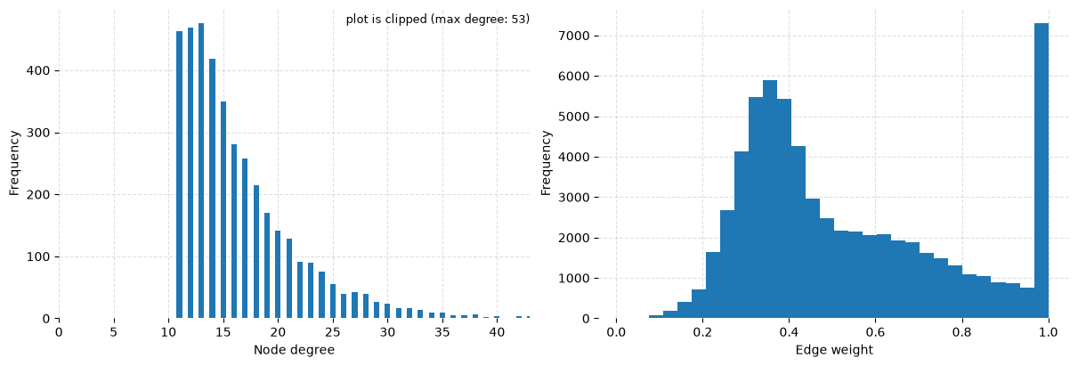
Started: 2026-10-11T18:55:46.669412Z | Wall time: 0.501 s
Check isolation and whether degree tracks QC metrics before treating the graph as ready for clustering:
# Count the neighbors connected to each cell.
degrees = np.asarray((loaded_graph != 0).sum(axis=0)).ravel()

# Summarize graph coverage and isolated cells.
pd.Series(
    {
        "active cells": int(loaded_graph.shape[0]),
        "isolated cells": int((degrees == 0).sum()),
        "median degree": float(np.median(degrees)),
        "min degree": int(degrees.min()),
        "max degree": int(degrees.max()),
    },
    name="graph coverage",
)
active cells 3948.0
isolated cells 0.0
median degree 15.0
min degree 11.0
max degree 53.0
Name: graph coverage, dtype: float64Started: 2026-10-11T18:55:47.174490Z | Wall time: 0.014 s
# Align graph degrees with the same cells' quality measurements.
degree_vs_qc = pd.DataFrame(
    {
        "degree": degrees,
        "RNA_nCounts": run_cells.fetch("RNA_nCounts"),
        "RNA_nFeatures": run_cells.fetch("RNA_nFeatures"),
    }
)

# Check whether graph degree tracks the quality measurements.
degree_vs_qc.corr(numeric_only=True)| degree | RNA_nCounts | RNA_nFeatures | |
|---|---|---|---|
| degree | 1.000000 | 0.077002 | 0.015492 |
| RNA_nCounts | 0.077002 | 1.000000 | 0.877195 |
| RNA_nFeatures | 0.015492 | 0.877195 | 1.000000 |
Started: 2026-10-11T18:55:47.191820Z | Wall time: 0.070 s
The graph should contain a row for every selected cell, with finite positive weights on its stored connections. Zero entries mean there is no edge between those cells. The degree summary detects isolated cells, but a graph with no isolated cells can still contain separate components.
Separate components can represent distinct populations. Investigate unexpected fragmentation
or a strong relationship between degree and QC metrics using markers, feature selection, PCA
dimensions, and k. Increasing k just to join every component can connect unrelated cells.
Use the graph for a layout and clustering
embeddings.umap and embeddings.tsne require both the graph and its matching initialization.
Leiden and Paris require the graph.
Each returns an immutable artifact without adding cell-metadata columns. Use
clusters.load_paris(ref) only when hierarchy diagnostics are needed.
Resolution 0.5 matches the prepared PBMC analysis; Leiden’s default is 1.0.
# Build starting coordinates for the embedding.
initialization = ds.embeddings.initialization(pca)

# Calculate the UMAP coordinates from the graph.
umap = ds.embeddings.umap(graph, initialization)

# Find groups of cells in the graph.
clusters = ds.clusters.leiden(graph, resolution=0.5)

# Read cluster labels in the selected cells' order.
cluster_values = np.asarray(ds.artifacts.load(clusters)["values"][:])

# Color the graph-derived UMAP by its Leiden clusters.
ds.plots.embedding(layout=umap, color_by=clusters)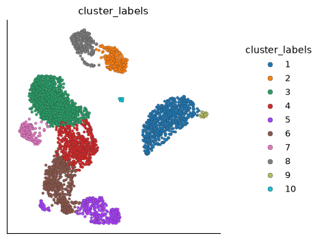
Started: 2026-10-11T18:55:47.265201Z | Wall time: 6.197 s
Branch by retaining both references
Suppose PCA and the approximate nearest-neighbor (ANN) index are expensive to recompute, but
you want to compare two neighbor counts. Query the same index with a different k: only the
neighbor and connectivity stages need new results. Keep both graph references so either analysis
can continue independently.
# Query the same index with 21 neighbors per cell.
neighbors_k21 = ds.graph.neighbors(ann_index, k=21)

# Build connectivity for the 21-neighbor comparison.
graph_k21 = ds.graph.connectivity(neighbors_k21)

# Check that the changed parameters produced a distinct result.
graph_k21 != graphTrueStarted: 2026-10-11T18:55:53.466002Z | Wall time: 0.496 s
Both branches remain complete, addressable artifacts. Downstream calls must receive one of them explicitly, so a parameter experiment cannot silently replace another branch.
Degree and edge weight both shift when every cell sees more neighbours:
# Load the comparison graph with symmetric edges.
loaded_graph_k21 = ds.graph.load(graph_k21, symmetric=True)

# Compare the number of stored edges in the two graphs.
pd.Series(
    {
        "k=11 nnz": int(loaded_graph.nnz),
        "k=21 nnz": int(loaded_graph_k21.nnz),
    },
    name="edges",
)
k=11 nnz 64990
k=21 nnz 122020
Name: edges, dtype: int64Started: 2026-10-11T18:55:53.965772Z | Wall time: 0.154 s
# Inspect graph degree and edge-weight distributions.
splt.graph_qc(loaded_graph_k21)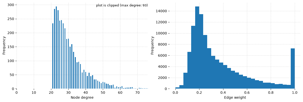
Started: 2026-10-11T18:55:54.124102Z | Wall time: 0.469 s
To analyse the side branch, pass its exact graph reference. Retain both returned refs so neither branch replaces the other.
# Cluster the 21-neighbor graph at the same resolution.
clusters_k21 = ds.clusters.leiden(graph_k21, resolution=0.5)

# Read the comparison cluster labels.
cluster_values_k21 = np.asarray(ds.artifacts.load(clusters_k21)["values"][:])

# Count cells in each reported category.
pd.Series(cluster_values_k21, name="cluster").value_counts().sort_index()
cluster
1 717
2 24
3 239
4 1312
5 353
6 319
7 564
8 149
9 256
10 15
Name: count, dtype: int64Started: 2026-10-11T18:55:54.596356Z | Wall time: 0.255 s
Place both partitions on the shared k=11 UMAP so changes in group boundaries are visible,
then compare their assignments with a crosstab:
# Create axes for the comparison panels.
figure, axes = plt.subplots(1, 2, figsize=(10, 4))

# Draw each result on its comparison axes.
for axis, cluster_ref, title in zip(
    axes,
    (clusters, clusters_k21),
    ("k=11 Leiden", "k=21 Leiden"),
    strict=True,
):

    # Compare the two clusterings on the same k=11 UMAP.
    ds.plots.embedding(
        layout=umap,
        color_by=cluster_ref,
        target=axis,
        show_titles=False,
        show=False,
    )

    # Label the panel with the result it shows.
    axis.set_title(title)

# Adjust spacing between the comparison panels.
figure.tight_layout()

# Display the completed comparison figure.
figure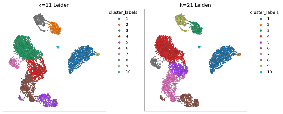
Started: 2026-10-11T18:55:54.854561Z | Wall time: 1.150 s
# Count cells shared by each pair of cluster assignments.
pd.crosstab(
    pd.Series(cluster_values, name="k=11"),
    pd.Series(cluster_values_k21, name="k=21"),
)| k=21 | 1 | 2 | 3 | 4 | 5 | 6 | 7 | 8 | 9 | 10 |
|---|---|---|---|---|---|---|---|---|---|---|
| k=11 | ||||||||||
| 1 | 716 | 0 | 0 | 0 | 0 | 0 | 0 | 0 | 0 | 0 |
| 2 | 0 | 0 | 239 | 0 | 0 | 0 | 0 | 0 | 0 | 0 |
| 3 | 0 | 0 | 0 | 1237 | 0 | 0 | 0 | 0 | 0 | 0 |
| 4 | 0 | 0 | 0 | 75 | 353 | 0 | 78 | 0 | 0 | 0 |
| 5 | 0 | 0 | 0 | 0 | 0 | 318 | 0 | 0 | 0 | 0 |
| 6 | 0 | 0 | 0 | 0 | 0 | 1 | 486 | 0 | 0 | 0 |
| 7 | 0 | 0 | 0 | 0 | 0 | 0 | 0 | 149 | 0 | 0 |
| 8 | 0 | 0 | 0 | 0 | 0 | 0 | 0 | 0 | 256 | 0 |
| 9 | 1 | 24 | 0 | 0 | 0 | 0 | 0 | 0 | 0 | 0 |
| 10 | 0 | 0 | 0 | 0 | 0 | 0 | 0 | 0 | 0 | 15 |
Started: 2026-10-11T18:55:56.008046Z | Wall time: 0.025 s
Cluster numbers can change even when the groups stay the same. Look for a row spread across
several columns, or a column collecting several rows, to find splits or merges that depend on
k. Review marker evidence before accepting those boundaries.
Recompute only what changed
Artifact identity includes the operation, scientific parameters, upstream inputs, and the operation’s revision.
Calling an identical stage reuses its completed result.
Changing k reuses normalization, PCA, and the ANN index but creates new neighbour and connectivity artifacts.
Changing the cell or feature selection requires new downstream results. The saved results of
the earlier analysis remain available.
Harmony changes the coordinates used to measure similarity. It reuses the existing PCA result, but its corrected coordinates need a new ANN index, neighbor search, and connectivity graph. Use it only when the study design supports technical batch correction:
# Correct PCA coordinates using a technical batch column.
corrected = ds.reduction.harmony(pca, ["technical_batch"])

# Build the neighbor index from corrected coordinates.
corrected_index = ds.graph.ann_index(corrected)

# Find neighbors in the corrected space.
corrected_neighbors = ds.graph.neighbors(corrected_index, k=21)

# Build connectivity from the corrected neighbors.
corrected_graph = ds.graph.connectivity(corrected_neighbors)
Use Why CyteArc records provenance to inspect complete lineage and Reuse results and compare analysis settings for reuse and invalidation patterns.