CyteArc keeps counts, metadata, graphs, and saved analysis results in a Zarr store. It reads count blocks as needed, so working with a datastore does not require loading the complete expression matrix into memory. Cell and feature metadata describe the rows and columns of that matrix.
This page starts with metadata queries and cell selections, then shows where counts and saved
results live. The examples require CyteArc’s extra optional dependencies.
Low-level layout details for contributors live in Zarr internals.
Open a prepared pancreas dataset
DataStore is the main entry point.
Each assay owns feature metadata, normalization, and feature selection.
Cell-level columns are shared across assays. The Boolean cell column I marks the active cells
used by live-metadata methods. Saved runs keep their own frozen cell selection.
Every assay spans all cells of the store. When an assay measured only some of them, as after a
merge of sources with different assays, the Boolean column <assay>_I, such as ADT_I, marks the
cells it measured; the other cells hold zero counts for that assay. Without that column, the assay
measured every cell. Those zero counts are no measurement, so an operation that reads an assay’s
values, such as normalization or marker search, refuses its unmeasured cells: select the measured
ones first with ds.select_measured_cells("ADT", cell_selection=...). Plots show the values of
unmeasured cells as missing.
The default assay supplies method defaults when from_assay is omitted.
It does not merge assay-specific feature tables or results.
# Import CyteArc and pandas to inspect the store and its metadata tables.
import pandas as pd

import cytearc

# Keep routine progress messages out of the teaching output.
cytearc.configure_output(level="WARNING", progress=False)
Started: 2026-10-11T18:54:45.876865Z | Wall time: 0.954 s
This page uses the pre-analyzed Bastidas-Ponce pancreas store also used in Core plotting features and Score cell-cycle activity.
It contains a completed pipeline run named docs_default. Opening this run gives us its
saved cell selection, computed clusters, and UMAP without running the analysis again.
# Download the prepared example, including its saved analysis.
dataset = cytearc.cytebase.connect("cytearc_docs").download_dataset(
    name="bastidas-ponce_4K_pancreas-d15_rnaseq",
    destination="cytearc_datasets",
    zarr=True,
)
Started: 2026-10-11T18:54:46.833999Z | Wall time: 3.206 s
Open the downloaded store and its saved analysis.
# Open the datastore for the following analysis.
ds = cytearc.DataStore(f"{dataset}/data.zarr", nthreads=4)

# Reuse the saved run and its frozen cell selection.
analysis_run = ds.pipeline.open(label="docs_default")

# Inspect the store's assays and dimensions.
ds
DataStore has 3696 (3696) cells with 1 assays: RNA
Cell metadata:
'I', 'ids', 'names', 'G2M_score', 'RNA_UMAP1',
'RNA_UMAP2', 'RNA_clusters', 'RNA_leiden_cluster', 'RNA_nCounts', 'RNA_nFeatures',
'RNA_percentMito', 'RNA_percentRibo', 'S_score', 'clusters', 'clusters_coarse'
RNA assay has 27998 features and following metadata:
'I', 'ids', 'names', 'dropOuts', 'highly_variable_genes',
'nCells'Started: 2026-10-11T18:54:50.048795Z | Wall time: 5.533 s
# Read the cluster labels in the run's cell order.
cluster_values = analysis_run.cells.fetch("clusters")

# Count cells in each cluster saved by the run.
cluster_counts = pd.Series(cluster_values, name="cluster").value_counts()

# Inspect cluster sizes in label order.
cluster_counts.sort_index().to_frame("cells")| cells | |
|---|---|
| cluster | |
| 1 | 378 |
| 2 | 546 |
| 3 | 493 |
| 4 | 215 |
| 5 | 223 |
| 6 | 340 |
| 7 | 205 |
| 8 | 145 |
| 9 | 93 |
| 10 | 500 |
| 11 | 315 |
| 12 | 243 |
Started: 2026-10-11T18:54:55.585343Z | Wall time: 0.149 s
The selected clustering remains in its exact artifact. The catalog’s literal clusters column is
an imported cell-type annotation, not a copy of this analytical result. Opening the run does not
modify either one.
Read cell and feature metadata
Cell and feature tables are MetaData objects (ds.cells, ds.RNA.feats), not pandas DataFrames.
Use head for a quick look, to_pandas_dataframe to export selected columns, and fetch / fetch_all for single columns.
# Preview cell identity, active status and the published annotation.
ds.cells.head()[["ids", "I", "clusters"]]| ids | I | clusters | |
|---|---|---|---|
| 0 | AAACCTGAGAGGGATA | True | Pre-endocrine |
| 1 | AAACCTGAGCCTTGAT | True | Ductal |
| 2 | AAACCTGAGGCAATTA | True | Alpha |
| 3 | AAACCTGCATCATCCC | True | Ductal |
| 4 | AAACCTGGTAAGTGGC | True | Ngn3 high EP |
Started: 2026-10-11T18:54:55.737534Z | Wall time: 0.150 s
# Preview the RNA feature metadata.
ds.RNA.feats.head()| I | ids | names | dropOuts | highly_variable_genes | nCells | |
|---|---|---|---|---|---|---|
| 0 | True | Xkr4 | Xkr4 | 3690 | False | 6 |
| 1 | True | Gm37381 | Gm37381 | 3696 | NaN | 0 |
| 2 | True | Rp1 | Rp1 | 3696 | NaN | 0 |
| 3 | True | Rp1-1 | Rp1-1 | 3696 | NaN | 0 |
| 4 | True | Sox17 | Sox17 | 3696 | NaN | 0 |
Started: 2026-10-11T18:54:55.893672Z | Wall time: 0.085 s
# Read selected QC columns alongside the published annotations.
cell_qc = ds.cells.to_pandas_dataframe(
    columns=["ids", "RNA_nCounts", "RNA_nFeatures", "clusters"]
)

# Preview the QC table with cell IDs as its row labels.
cell_qc.set_index("ids").head()| RNA_nCounts | RNA_nFeatures | clusters | |
|---|---|---|---|
| ids | |||
| AAACCTGAGAGGGATA | 4954.0 | 2356.0 | Pre-endocrine |
| AAACCTGAGCCTTGAT | 7071.0 | 2613.0 | Ductal |
| AAACCTGAGGCAATTA | 4070.0 | 1984.0 | Alpha |
| AAACCTGCATCATCCC | 8362.0 | 2860.0 | Ductal |
| AAACCTGGTAAGTGGC | 5026.0 | 2211.0 | Ngn3 high EP |
Started: 2026-10-11T18:54:55.981735Z | Wall time: 0.068 s
insert writes a new column and aligns values to the active subset unless you override key.
When the values cover only the rows that key selects, the other rows are missing: they are
flagged in the column’s missing mask, to_pandas_dataframe and plots show them as missing, and
sift never selects them. Pass fill_value to store a real value in those rows instead; it must
fit the values, such as False for a Boolean column. None, NaN, and pd.NA among the
values are missing too. Re-inserting an existing column requires overwrite=True, and a failed
replacement keeps the previous column.
In this prepared store, every cell is active and the saved run contains the same cells, so its
cluster labels align with the values we insert. For another analysis, check the cell selection
before copying results into live metadata.
# Choose the cluster containing the first selected cell.
first_run_cluster = cluster_values[0]

# Mark cells belonging to that cluster.
is_first_cluster = cluster_values == first_run_cluster

# Save the values in cell metadata using the stated selection.
ds.cells.insert(
    column_name="is_first_cluster", values=is_first_cluster, overwrite=True
)

# Check the sizes of the selected cluster and its complement.
pd.Series(is_first_cluster).value_counts().rename("cells")
False 3318
True 378
Name: cells, dtype: int64Started: 2026-10-11T18:54:56.051868Z | Wall time: 0.028 s
# Preview the newly saved cluster-selection column.
ds.cells.to_pandas_dataframe(
    columns=["ids", "clusters", "is_first_cluster"]
).head()| ids | clusters | is_first_cluster | |
|---|---|---|---|
| 0 | AAACCTGAGAGGGATA | Pre-endocrine | True |
| 1 | AAACCTGAGCCTTGAT | Ductal | False |
| 2 | AAACCTGAGGCAATTA | Alpha | False |
| 3 | AAACCTGCATCATCCC | Ductal | False |
| 4 | AAACCTGGTAAGTGGC | Ngn3 high EP | False |
Started: 2026-10-11T18:54:56.082460Z | Wall time: 0.054 s
# Locate the selected cluster on the saved UMAP.
ds.plots.embedding(layout=analysis_run["umap"], color_by="is_first_cluster")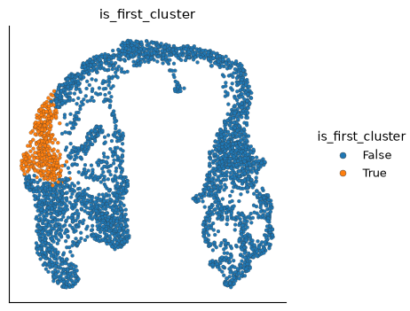
Started: 2026-10-11T18:54:56.140178Z | Wall time: 1.619 s
The new column marks one cluster on the same active cells used for the insert.
fetch returns values for the active subset (default column I).
fetch_all returns every row in the store.
With every cell active the lengths match. Pass the new Boolean column as key to select one
cluster without changing I:
# Compare a selected fetch with the complete metadata axis.
print(
    "fetch:",
    ds.cells.fetch("clusters", key="is_first_cluster").shape,
    "fetch_all:",
    ds.cells.fetch_all("clusters").shape,
)
fetch: (378,) fetch_all: (3696,)
Started: 2026-10-11T18:54:57.762503Z | Wall time: 0.024 s
Select cells from metadata
sift returns a boolean mask over all metadata rows for one numeric range. Its bounds are
exclusive by default: the next call selects cells with more than 1,000 and fewer than 15,000
counts. Pass keep_bounds=True to include the endpoints.
multi_sift keeps rows that satisfy every range, with one lower and one upper bound per
column. get_index_by returns row indexes for exact categorical matches:
# Record the active-cell count before creating new masks.
active_before = int(ds.cells.fetch_all("I").sum())

# Select cells within the stated count range.
count_range = ds.cells.sift("RNA_nCounts", min_v=1000, max_v=15000)

# Count cells inside the count range.
{"cells in count range": int(count_range.sum())}
{'cells in count range': 3669}Started: 2026-10-11T18:54:57.789189Z | Wall time: 0.015 s
Combine count and detected-gene limits.
# Apply count and detected-feature ranges together.
joint_range = ds.cells.multi_sift(
    columns=["RNA_nCounts", "RNA_nFeatures"],
    lows=[1000, 500],
    highs=[15000, 4000],
)

# Count cells satisfying both QC ranges.
{"cells in both QC ranges": int(joint_range.sum())}
{'cells in both QC ranges': 3667}Started: 2026-10-11T18:54:57.806441Z | Wall time: 0.016 s
Find rows by their published annotation.
# Find the physical rows annotated as ductal cells.
ductal_rows = ds.cells.get_index_by(["Ductal"], "clusters")

# Count the rows matching the published ductal annotation.
print("Ductal cells:", int(ductal_rows.size))

# Show the active-cell count recorded before creating masks.
print("Active cells (I) before:", active_before)

# Check that creating masks left the active selection unchanged.
print("Active cells (I) after:", int(ds.cells.fetch_all("I").sum()))
Ductal cells: 916
Active cells (I) before: 3696
Active cells (I) after: 3696
Started: 2026-10-11T18:54:57.825516Z | Wall time: 0.024 s
# Save the values in cell metadata using the stated selection.
ds.cells.insert(column_name="in_count_range", values=count_range, overwrite=True)

# Locate cells inside the count range on the saved UMAP.
ds.plots.embedding(layout=analysis_run["umap"], color_by="in_count_range")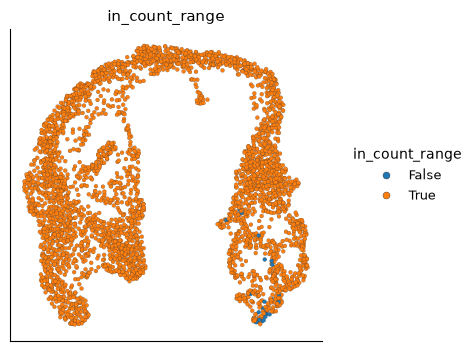
Started: 2026-10-11T18:54:57.851838Z | Wall time: 0.461 s
These helpers return masks or indexes aligned with the metadata table.
They do not modify I until you explicitly insert or update a cell key.
See the MetaData API in Assays and metadata API reference for update and delete helpers.
Optional: inspect counts and saved results
The metadata examples above are enough to read annotations and select cells. Continue here when you need to inspect the underlying arrays or understand where analysis results are stored.
Count matrices and normalization
Raw counts are a Zarr array (often sharded), exposed as rawData, a chunked array with a NumPy-like interface that streams by row.
In this store the array is at RNA/counts.
RNA assays also store countsT, a gene-major copy used by HVG and marker stages.
Routine analysis does not need to touch either array directly.
Normalized values are computed on demand through the lower-level assay normed() view from raw counts.
features.normalize(cell_selection, features) is the public persisted path and requires exact stored cell- and feature-selection references.
The direct normed() view follows its explicit or literal metadata indexes; in a newly created
store the physical feature I column is all true. Inspect the shapes without loading the
complete matrix:
# Inspect raw matrix dimensions without reading its values.
print("Raw shape:", ds.RNA.rawData.shape)

# Inspect normalized-view dimensions without materializing the matrix.
print("Normed shape:", ds.RNA.normed().shape)
Raw shape: (3696, 27998)
Normed shape: (3696, 27998)
Started: 2026-10-11T18:54:58.319524Z | Wall time: 0.034 s
For a worked example that reads count blocks for an external calculation, see Extending CyteArc with custom analyses.
Inspect saved analysis results
Analysis methods return lightweight references to results stored in Zarr.
The completed docs_default run retained the HVG and normalization references it created.
Asking for the same normalization again reuses that result rather than recomputing:
# Request the saved normalization using the same exact inputs.
reused_normalized = ds.features.normalize(
    analysis_run["analysis_cell_selection"],
    analysis_run["highly_variable_features"],
)

# Check whether this request reused the saved normalization.
print("Reused:", reused_normalized == analysis_run["normalized"])

# Inspect the reference identifying the reused normalization.
reused_normalized
Reused: True
ArtifactRef(assay='RNA', kind='normalized', artifact_id='9fb6d37118da...')Started: 2026-10-11T18:54:58.355654Z | Wall time: 0.148 s
Inspect its status and open the underlying group only when a custom method needs direct access:
# Inspect the saved result's completeness and provenance.
status = ds.artifacts.inspect(reused_normalized)

# Check that the saved normalization is complete.
print("Complete:", status.complete)

# Show the operation that created this artifact.
print("Operation:", status.operation)

# Show the normalization method without its internal registration details.
print("Method:", status.parameters["normalization_method"]["qualname"])

# Keep the numerical and transformation settings used for this result.
normalization_settings = {
    key: status.parameters[key]
    for key in ("size_factor", "log_transform", "renormalize_subset")
}

# Open the artifact arrays for a low-level inspection.
group = ds.artifacts.load(reused_normalized)

# List a few arrays available in the saved artifact.
print("Arrays:", list(group.array_keys())[:5])

# Inspect one normalization setting per row.
pd.Series(normalization_settings, name="value").rename_axis("setting").to_frame()
Complete: True
Operation: run_normalization
Method: norm_lib_size
Arrays: ['data', 'feature_m2', 'feature_sum']
| value | |
|---|---|
| setting | |
| size_factor | 1000.0 |
| log_transform | True |
| renormalize_subset | True |
Started: 2026-10-11T18:54:58.506628Z | Wall time: 0.025 s
Identical inputs and parameters reuse a complete result. Branching, invalidation, and lineage are covered in Reuse results and compare analysis settings.
Look inside the store
CyteArc uses Zarr for chunked on-disk arrays. The store is a directory tree: counts, cell and feature attributes, and immutable artifacts live under named groups. Each array has its own shape, dtype, and chunk layout. CyteArc reads and writes those chunks without loading every array in the store.
show_zarr_tree prints the hierarchy.
With depth=0 you see the top-level assays and cellData.
# Locate the top-level assays, metadata and saved analyses.
ds.show_zarr_tree(depth=0)
/
├── RNA
├── artifacts
├── cellData
└── pipeline
Started: 2026-10-11T18:54:58.534248Z | Wall time: 0.016 s
Cell statistics computed from an assay are stored under cellData with the assay name as a prefix (RNA_…, ADT_…).
# Inspect the storage layout of the active-cell flag and two QC columns.
metadata_arrays = {
    name: ds.zw["cellData"][name]
    for name in ("I", "RNA_nCounts", "RNA_nFeatures")
}

# Compare array shapes, value types and chunk sizes without loading values.
pd.DataFrame({
    name: {
        "shape": array.shape,
        "dtype": str(array.dtype),
        "chunks": array.chunks,
    }
    for name, array in metadata_arrays.items()
}).T.rename_axis("cellData column")| shape | dtype | chunks | |
|---|---|---|---|
| cellData column | |||
| I | (3696,) | bool | (100000,) |
| RNA_nCounts | (3696,) | float64 | (100000,) |
| RNA_nFeatures | (3696,) | float64 | (100000,) |
Started: 2026-10-11T18:54:58.552642Z | Wall time: 0.020 s
The I column is the default user-owned cell key, tracking which cells are active for
live-metadata APIs. Values are boolean.
Use snapshot_cell_selection("I") to capture this live column before passing it to an analytical
producer. Some metadata, mapping, and export utilities still accept cell_key directly.
# Count active and inactive rows on the complete cell axis.
ds.cells.to_pandas_dataframe(["I"])["I"].value_counts()
I
True 3696
Name: count, dtype: int64Started: 2026-10-11T18:54:58.575712Z | Wall time: 0.026 s
This store keeps every barcode active (True). Analytical filtering returns a separate immutable
selection artifact and leaves this column unchanged. If you deliberately author a live selection
column, its False rows also remain in the table rather than being deleted.
Each assay group holds featureData and its persisted artifacts.
Count matrices are Zarr arrays, often sharded. This store keeps RNA counts at RNA/counts.
# Inspect this part of the store hierarchy without reading counts.
ds.show_zarr_tree(start="RNA", depth=1)
/RNA
├── artifacts
│ ├── ann_index
│ ├── cluster_labels
│ ├── cluster_selection
│ ├── connectivity_map
│ ├── embedding
│ ├── embedding_initialization
│ ├── feature_scaling
│ ├── feature_selection
│ ├── feature_summary
│ ├── marker_table
│ ├── metadata_snapshot
│ ├── neighbors
│ ├── normalized
│ └── reduction
├── countSummaries
│ ├── columnPositive (27998,) int64
│ ├── featureSums
│ ├── rowPositive (3696,) int64
│ └── rowSums (3696,) float64
├── counts (3696, 27998) uint16
├── countsT (27998, 3696) uint16
└── featureData
├── I (27998,) bool
├── __cytearc_missing__highly_variable_genes (27998,) bool
├── dropOuts (27998,) int64
├── highly_variable_genes (27998,) <U5
├── ids (27998,) <U15
├── nCells (27998,) int64
└── names (27998,) <U15
countsT: shape=(27998, 3696), dtype=uint16, chunks=(27056, 1848), shards=(27056, 3696)
counts: shape=(3696, 27998), dtype=uint16, chunks=(3696, 13528), shards=(3696, 40584)
Started: 2026-10-11T18:54:58.605415Z | Wall time: 0.037 s
For feature arrays, pass start="RNA/featureData" to the same method.
Each persisted result is an artifact. Assay-scoped results live under
{assay}/artifacts/{kind}/{artifact_id}; datastore-scoped selections and integrated results live
under artifacts/{kind}/{artifact_id}.
The kind names the operation family and the identifier is random; CyteArc recognises an equivalent result by its recorded operation, revision, parameters, and inputs instead of recomputing it.
Nothing here encodes parameters in the path, so a second PCA at different dimensionality becomes a sibling entry rather than a new branch of the tree.
To inspect saved result groups, use ds.show_zarr_tree(start="RNA/artifacts", depth=1).
Zarr internals covers the complete on-disk layout.
Zarr versions and storage profiles
Current CyteArc versions write new datasets as Zarr v3.
RNA assays also write a gene-major countsT copy next to counts.
The catalog dataset used here was rebuilt from its raw source with this codebase, so it already has
the current layout. Re-import older RNA stores that use Zarr v2 or lack countsT before analysis.
Count matrices from the writers use sharded arrays (default profile fast_local).
Set the profile with CYTEARC_ZARR_PROFILE (fast_local or cloud) or zarrProfile= when opening a DataStore.
Storage profiles and conversion belong to the physical store, while mem_budget and nthreads control execution.
See Memory and execution for why RNA stores two orientations, and Explore a remote dataset for object storage and local scratch.
Common mistakes and limitations
Treating on-disk objects as in-memory ones:
MetaDatais not a pandas DataFrame;fetchreturns rows selected byIby default, whilefetch_allreturns every row, and an analysis result is a stored artifact, not a matrix to index directly.Expecting filtering to delete cells or edit saved results: filtering never deletes rows or rewrites live
I, and saved artifacts are immutable products of analysis methods, not groups to edit by hand.Opening an older RNA store (Zarr v2, or without the
countsTcopy) in a current CyteArc version; re-import the store before analysis.
Metadata changes and artifacts are written into the Zarr store. Low-level layout details intended for contributors remain in Zarr internals.