Explore a remote dataset

Open a shared dataset, inspect a few genes, and save your own work without copying the count matrix. This example uses Tabula Sapiens: 1,136,218 cells from 24 donors. You need an internet connection and CyteArc’s extra dependencies; no credentials are required.

Start with a read-only connection for questions and plots. Create a writable mount later, when you want to save annotations or analysis results. Each code cell shows its measured wall time below the output; network access and the number of points drawn affect that time.

Open the published analysis¶

Open the remote store read-only and find the authors’ UMAP:

# Import CyteArc and keep progress output out of the figures.
import cytearc
from cytearc.plotting import CategoricalScale, CellField, ColorScale, NormalizationSpec

cytearc.configure_output(level="ERROR", progress=False)

Started: 2026-10-11T18:54:52.018001Z | Wall time: 1.347 s

# Open the full atlas without downloading the dataset archive.
source_uri = "hf://buckets/Nygen/cytebase/cytearc_docs/tabula_sapiens/data.zarr"
source = cytearc.DataStore(
    source_uri,
    zarr_mode="r",
    storage_options={"token": False},
    min_features_per_cell=-1,
)

# Find the UMAP imported from the authors' dataset.
author_umap = cytearc.cytebase.embedding(source)

Started: 2026-10-11T18:54:53.367693Z | Wall time: 7.492 s

Inspect one population¶

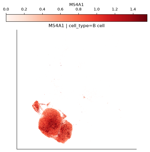
Start with MS4A1, a B-cell marker, in cells annotated as B cells by the authors. facet_by and groups restrict the plot to that population without writing a selection or creating a mount. The published UMAP supplies the coordinates:

# Read MS4A1 expression for the author-annotated B cells.
source.plots.embedding(
    layout=author_umap,
    color_by="MS4A1",
    facet_by="cell_type",
    groups=["B cell"],
    normalization=NormalizationSpec(transform="log1p"),
    color_scale=ColorScale(cmap="Reds", quantiles=(0, 0.99)),
    sort_values=True,
    point_size=0.5,
    figsize=(6, 5),
)

Published Tabula Sapiens UMAP restricted to 114,495 author-annotated B cells, coloured by log1p MS4A1 expression on a red scale capped at the 99th percentile.

Started: 2026-10-11T18:55:00.862325Z | Wall time: 17.794 s

The plot contains the 114,495 author-annotated B cells. CyteArc reads the saved layout and the count blocks needed for their expression values. The complete expression matrix stays in object storage.

Compare with the full atlas¶

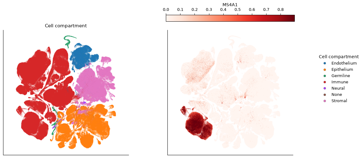
For context, compare the major cell compartments with MS4A1 expression across all 1.1 million cells. Drawing two panels at this size takes longer than drawing one population:

# Use the authors' UMAP for both compartments and marker expression.
source.plots.embedding(
    layout=author_umap,
    color_by=[CellField("compartment", kind="categorical", label="Cell compartment"), "MS4A1"],
    normalization=NormalizationSpec(transform="log1p"),
    color_scale=ColorScale(cmap="Reds", quantiles=(0, 0.99)),
    sort_values=True,
    point_size=0.2,
    n_columns=2,
    figsize=(12, 5),
    legend_loc="right",
)

Two panels show the full Tabula Sapiens UMAP by cell compartment and log1p MS4A1 expression. Strong MS4A1 signal is concentrated in a region of the immune compartment.

Started: 2026-10-11T18:55:18.658403Z | Wall time: 25.060 s

The UMAP and compartment labels come from the authors. CyteArc reads the coordinates and metadata, then reads count blocks for the gene panel and displays log-normalized expression. The color scale saturates at the 99th percentile to make expression easier to see. Computation runs in your Python session, and the complete count matrix stays in object storage. Use additional markers before assigning cell types; see Annotate cell types and states.

Save a cell selection locally¶

A mount gives you a writable store for metadata and new results while leaving counts at their source. Several people can mount the same published dataset and keep separate analyses. The source can be local or remote; here it is remote and the target is a local directory. Mounting copies metadata and takes more work than opening the source read-only. Choose a new or empty path for the target:

# Create a local place for annotations and new analysis results.
mounted = cytearc.mount_datastore(
    source_uri,
    at="tabula_analysis.zarr",
    storage_options={"token": False},
    min_features_per_cell=-1,
)

# Select cells annotated as B cells by the authors.
selected = mounted.cells.fetch_all("cell_type") == "B cell"
mounted.cells.insert("b_cells", selected)

# Check that the selection is present, then count its cells.
assert selected.any()
{"B cells selected": int(selected.sum())}

{'B cells selected': 114495}

Started: 2026-10-11T18:55:43.721338Z | Wall time: 15.625 s

Cell and feature metadata are copied into tabula_analysis.zarr; count matrices remain in the published store. Your b_cells column is local. Other people can mount the same source and keep their own selections and results.

Reopen your work¶

Open the local path again. It remembers where to read the counts:

# Reopen the local mount with anonymous access to its public count source.
reopened = cytearc.DataStore(
    "tabula_analysis.zarr",
    storage_options={"token": False},
    min_features_per_cell=-1,
)

# Open the source afresh to check that its metadata was not changed.
fresh_source = cytearc.DataStore(
    source_uri,
    zarr_mode="r",
    storage_options={"token": False},
    min_features_per_cell=-1,
)

# Check that the selection persisted locally and did not appear in the source.
checks = {
    "selection preserved": bool((reopened.cells.fetch_all("b_cells") == selected).all()),
    "shared source unchanged": "b_cells" not in fresh_source.cells.columns,
}
assert all(checks.values()), checks
checks

{'selection preserved': True, 'shared source unchanged': True}

Started: 2026-10-11T18:55:59.348591Z | Wall time: 3.225 s

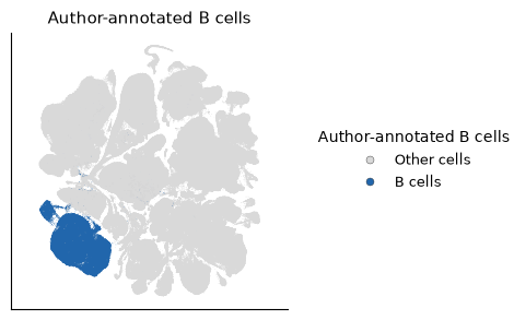
Both checks return True: the B-cell selection is saved locally and the source metadata is unchanged. The mount can also read saved artifacts from the source, including its UMAP, without copying them into the target:

# Display the local selection on the existing remote UMAP.
reopened.plots.embedding(
    layout=author_umap,
    color_by=CellField("b_cells", kind="categorical", label="Author-annotated B cells"),
    categorical_scale=CategoricalScale(
        palette={False: "#d9d9d9", True: "#2166ac"},
        labels={False: "Other cells", True: "B cells"},
    ),
    point_size=0.2,
    legend_loc="right",
)

Full Tabula Sapiens UMAP with the locally saved B-cell selection in blue and other cells in grey, using the original remote coordinates.

Started: 2026-10-11T18:56:02.576300Z | Wall time: 11.867 s

Keep tabula_analysis.zarr to return to your work. The remote source must remain accessible. Mounting saves a copy of the metadata, so later changes to the source’s annotations do not silently replace yours.

Continue with your analysis¶

Analyze the selected B cells: run mounted.pipeline.run(cell_key="b_cells", label="b_cells"). The RNA-seq pipeline reads their count blocks from the source and writes new results locally. Saving a selection alone does not change which cells the pipeline uses.
Find another dataset: search the Explore CyteBase, then follow the CyteBase case study: COVID-19 blood for a study with donor-level comparisons.
Connect your own storage: see Remote storage configuration for S3 and GCS access, source requirements, and local scratch settings.
Work offline: download the prepared 100,000-cell sample in the Quick start.