Pool cells into pseudobulk profiles

Tests of conditions compare samples, so the cells of every sample and cell type are first pooled into one profile (Why pseudobulk). A cube keeps those profiles: for every gene, sums over the cells of each sample and cell type, with the number of cells pooled into each. Because every value is a sum, cell types can be merged and samples pooled later without the cells, and the same sums give what describes the cells: the fraction that express each gene and their mean expression, the values of a dot plot. This page pools the cells of the simulated PBMC study (the simulated_pbmc dataset of the Datasets page), looks at the markers of its cell types and at its samples, and merges a rare cell type into its lineage. The cube and its additive layers defines every layer.

Samples, cell types and layers¶

from_cells takes a cells x genes matrix of counts and the sample and the cell type of every cell. A sample table, with a sample_id for every sample label, sets the order of the samples and carries the variables that designs use, here the donor and the condition; a group table does the same for the cell types, and may carry their lineage.

import matplotlib.pyplot as plt
import numpy as np
import scipy.sparse

import cytepool
from cytepool.cube import from_cells
from cytepool.plotting import plot_cell_numbers, plot_dotplot, plot_pca

cells = np.load("simulated_pbmc_cells.npz")
counts = scipy.sparse.csr_array(
    (cells["data"], cells["indices"], cells["indptr"]), shape=tuple(cells["shape"])
)
sample_ids = np.unique(cells["cell_sample"])
cube = from_cells(
    counts,
    samples=cells["cell_sample"],
    groups=cells["cell_type"],
    sample_table={
        "sample_id": sample_ids,
        "donor": [sample.split("_")[0] for sample in sample_ids],
        "condition": [sample.split("_")[1] for sample in sample_ids],
    },
    group_table={
        "group_id": cells["cell_types"],
        "lineage": ["lymphoid"] * 4 + ["myeloid"] * 2,
    },
    features=cells["feature_id"],
)
print(f"CytePool {cytepool.__version__}")
print(cube)
print(cube.groups)

CytePool 0.1.dev61+g194f49f8f
Cube with 24 samples x 6 groups x 2,000 features
  layers: counts (uint32), detected (uint32), log_sum (float64), log_sum_sq (float64), linear_sum (float64)
  filled: 144 of 144 sample x group entries have cells (100.0%)
  samples: sample_id, donor, condition
  groups: group_id, lineage
  features: feature_id
Table with 6 rows and 2 columns
  group_id         lineage
  str              str
  B cells          lymphoid
  CD4 T cells      lymphoid
  CD8 T cells      lymphoid
  NK cells         lymphoid
  Monocytes        myeloid
  Dendritic cells  myeloid

The cube holds five layers: the counts, which the tests read, and four that describe the cells: detected, the number of cells with a positive count, and the sums of the cells’ log-normalized values (log_sum), of their squares (log_sum_sq) and of the normalized values themselves (linear_sum). Each cell is normalized to 10,000 counts and log-transformed, as scanpy’s normalize_total and log1p do.

The markers of each cell type¶

A dot plot shows, for chosen genes and cell types, the fraction of the cells that express each gene, as the area of a dot, and their mean expression, as its colour, as scanpy draws it Wolf et al., 2018. plot_dotplot reads both from the cube, pooled over every sample, and gives the values scanpy computes from the cells (Validation). The simulation gave each cell type 20 marker genes; here are three of each, with the means of each gene scaled from 0 to 1 over the cell types, as scanpy’s standard_scale="var" scales them.

markers = {
    cell_type: list(genes[:3])
    for cell_type, genes in zip(cells["cell_types"], cells["marker_genes"])
}
ax = plot_dotplot(cube, markers, standard_scale="gene")
plt.show()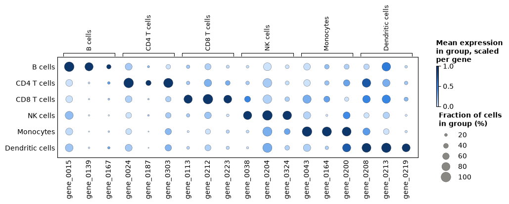

Dot plot of 18 marker genes (columns, three for each cell type, under a bracket that names it) in six cell types (rows): a dot's area gives the percentage of the cell type's cells that express the gene, from about 5 to 100, and its shade of blue their mean expression, scaled from 0 to 1 over the cell types for each gene. Each cell type's three markers have the darkest and largest dots of its row, under its own bracket; a few markers, such as gene_0204 of the NK cells and gene_0213 of the dendritic cells, are expressed in most cells of every type and are darkest in their own.

Each cell type’s markers are expressed in more of its cells, and more highly, than in the other cell types, as an annotation that is right shows them. A cell type whose markers light up in another row is worth a second look before any test.

What changes in the cells¶

Cube.collapse_samples pools the samples that share a value of a sample column, here the condition: the profiles of the 12 control samples are summed into one, and so are those of the 12 stimulated ones. From the pooled sums, Cube.fraction_detected, Cube.mean and Cube.variance give the fraction of the cells that detect each gene, and the mean and the variance of their log-normalized values. For one gene of the response program that the simulation gave every cell type:

by_condition = cube.collapse_samples("condition")
print(by_condition.samples)

gene = cube.features["feature_id"].tolist().index("gene_0191")
detected = by_condition.fraction_detected()[:, :, gene]
mean = by_condition.mean()[:, :, gene]
variance = by_condition.variance()[:, :, gene]
print(f"\ngene_0191, control -> stimulated{'detected':>12}{'mean':>16}{'variance':>16}")
for g, cell_type in enumerate(by_condition.groups["group_id"]):
    print(
        f"{cell_type:<32}{detected[g, 0]:>6.2f} -> {detected[g, 1]:.2f}"
        f"{mean[g, 0]:>8.2f} -> {mean[g, 1]:.2f}{variance[g, 0]:>8.2f} -> {variance[g, 1]:.2f}"
    )

Table with 2 rows and 3 columns
  sample_id  condition  n_pooled_samples
  str        str        int64
  ctrl       ctrl       12
  stim       stim       12

gene_0191, control -> stimulated    detected            mean        variance
B cells                           0.86 -> 1.00    1.98 -> 3.44    0.90 -> 0.43
CD4 T cells                       0.78 -> 0.99    1.59 -> 3.26    0.92 -> 0.48
CD8 T cells                       0.85 -> 0.99    1.87 -> 3.50    0.91 -> 0.49
NK cells                          0.74 -> 0.97    1.49 -> 2.89    0.98 -> 0.64
Monocytes                         0.65 -> 0.97    1.20 -> 2.88    0.92 -> 0.60
Dendritic cells                   0.75 -> 0.96    1.53 -> 2.78    0.97 -> 0.82

After the stimulation nearly every cell of every type expresses the gene, and the mean of their log-normalized values about doubles. These pooled values describe the cells; they are no test, since the samples pooled are the replicates a test needs (Genes that change in each cell type tests the change). Pooling the samples of each donor, collapse_samples("donor"), gives one profile per donor, for questions about donors (Repeated measures and donors).

The samples of each cell type¶

DESeq2’s PCA plot places the samples of one cell type on the principal components of their 500 most variable genes Love et al., 2014, prepared as for an MDS plot: profiles of fewer than 10 cells are left out, genes are filtered by expression, and the values are log-CPM (plot_pca, principal_components). It shows at a glance whether the samples group as the design expects.

figure, (left, right) = plt.subplots(1, 2, figsize=(12, 4.6), layout="constrained")
plot_pca(cube, group="Monocytes", color_by="condition", ax=left)
plot_pca(
    cube,
    group="Monocytes",
    color_by="condition",
    marker_by="donor",
    components=(2, 3),
    ax=right,
)
plt.show()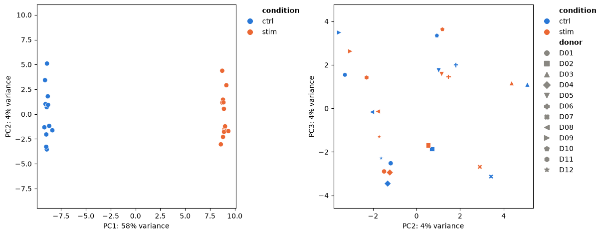

Two PCA plots of the 24 monocyte samples, coloured by condition (control blue, stimulated orange). Left, PC1 (58% of the variance) against PC2 (4%): the control samples lie near -9 on PC1 and the stimulated ones near 9. Right, PC2 against PC3 (4%), each donor with a marker of its own: the two samples of most donors lie next to each other, such as those of D09 at the top left, of D03 at the right and of D04 at the bottom.

The first component, more than half of the variance, is the stimulation. On the second and third, each donor’s two samples lie near each other: donors differ, which is why the design of Genes that change in each cell type pairs them.

A cell type with few cells¶

Six profiles of dendritic cells pool fewer than 10 cells, and limma_voom leaves them out of the dendritic cells’ fit (Quick start). Where a rare cell type matters less than its lineage, Cube.regroup merges it with related cell types: every layer of the merged cell type is the sum of its members’, as pooling the relabelled cells would give. Here the group table’s lineage names the myeloid cell types (Table.filter).

myeloid = cube.groups.filter(cube.groups["lineage"] == "myeloid")["group_id"]
merged = cube.regroup({"Myeloid cells": list(myeloid)})
print(merged.groups)
plot_cell_numbers(merged)
plt.show()

Table with 5 rows and 2 columns
  group_id       lineage
  str            str
  B cells        lymphoid
  CD4 T cells    lymphoid
  CD8 T cells    lymphoid
  NK cells       lymphoid
  Myeloid cells  myeloid

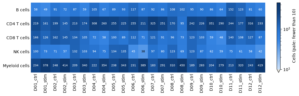
Heatmap of the cells pooled into each of the 24 samples and five cell types, after the monocytes and dendritic cells are merged into myeloid cells: the myeloid cells hold from 183 to 450 cells, and no entry is pale; the other rows are as before, with the fewest cells, 38, in the NK cells of D06_stim.

Every profile of the merged myeloid cells holds enough cells. The merged profile mixes two cell types in proportions that differ between samples, and the stimulation changes those proportions (Cell-type composition), so a change in the merged profile can come from either; testing the monocytes alone, and the dendritic cells on their 18 profiles, keeps the two apart.

Choices¶

Samples. A sample is a biological replicate: one donor in one condition, or one tissue of a donor. Pool technical replicates, such as lanes or libraries of the same sample, by giving them one sample label, or later with Cube.collapse_samples.
Tables. The sample and group tables take a pandas DataFrame or a mapping of columns, and a cube keeps them as Table objects: Table.select keeps some columns, Table.filter some rows, Table.with_columns adds columns, such as a variable for a design, and Table.to_pandas gives a DataFrame.
Cell types. Annotate at the level the question needs. Cube.select keeps some cell types, Cube.regroup merges them, and the minimum of cells (min_cells of limma_voom, 10 by default) leaves out the profiles of too few cells, with the reason in the result.
Layers. layers="counts" keeps only what the tests read: 4 bytes per sample, cell type and gene, against 32 for all five layers, which matters for atlases of thousands of samples. The dot plot needs detected and log_sum, and Cube.variance needs log_sum_sq.
Normalization of the cells. target_sum (10,000) sets the total that every cell is scaled to, and library_sizes gives the totals when the matrix holds only some of the genes.
Bulk data. from_bulk wraps a samples x genes matrix of counts as a cube with one group, which every test of a cube takes (Bulk RNA-seq).
Other tools. Cells in an AnnData, and profiles pooled by scanpy, decoupler or LIANA, become cubes too (Work with AnnData and MuData).

References¶

Wolf, F. A., Angerer, P., & Theis, F. J. (2018). SCANPY: large-scale single-cell gene expression data analysis. Genome Biology, 19(1), 15. 10.1186/s13059-017-1382-0
Love, M. I., Huber, W., & Anders, S. (2014). Moderated estimation of fold change and dispersion for RNA-seq data with DESeq2. Genome Biology, 15(12), 550. 10.1186/s13059-014-0550-8