Before testing, look at the data: do the samples group as the design expects, which
genes have enough counts to be tested, do the libraries need rescaling, and does any
sample or gene behave unlike the rest? limma_voom takes these steps inside,
with defaults; this page takes them one at a time, so that each choice can rest on
what the data show. It uses the CD14+ monocytes of the Kang data Kang et al., 2018 and the
simulated bulk experiment, whose noisier sample is known (the kang2018 and
simulated_bulk datasets of the Datasets page).
Do the samples group as expected?
limma’s multidimensional scaling plot (plot_mds) places the samples so that
their distances are the typical log2 fold changes between them, the root mean square
of the 500 largest. From a cube it takes one cell type’s counts, filtered and
normalized as edgeR prepares them for its own plot.
import matplotlib.pyplot as plt
import numpy as np

import cytepool
from cytepool.design import Design
from cytepool.differential_expression import limma_voom
from cytepool.io import read_cube
from cytepool.normalization import (
    filter_by_expression,
    median_ratio_size_factors,
    rle_factors,
    tmm_factors,
    upper_quartile_factors,
)
from cytepool.plotting import (
    plot_mds,
    plot_mean_variance,
    plot_residual_variances,
    plot_sample_weights,
)
from cytepool.stats.empirical_bayes import moderated_statistics
from cytepool.stats.linear_models import contrasts_fit, fit_linear_model
from cytepool.stats.voom import voom

kang = read_cube("kang2018.cube.zarr")
print(f"CytePool {cytepool.__version__}")
figure, (left, right) = plt.subplots(1, 2, figsize=(11, 4.2), layout="constrained")
for ax, dimensions in ((left, (1, 2)), (right, (2, 3))):
    plot_mds(
        kang,
        group="CD14+ Monocytes",
        color_by="condition",
        marker_by="donor",
        dimensions=dimensions,
        ax=ax,
    )
plt.show()
CytePool 0.1.dev54+g3f0cbb52e
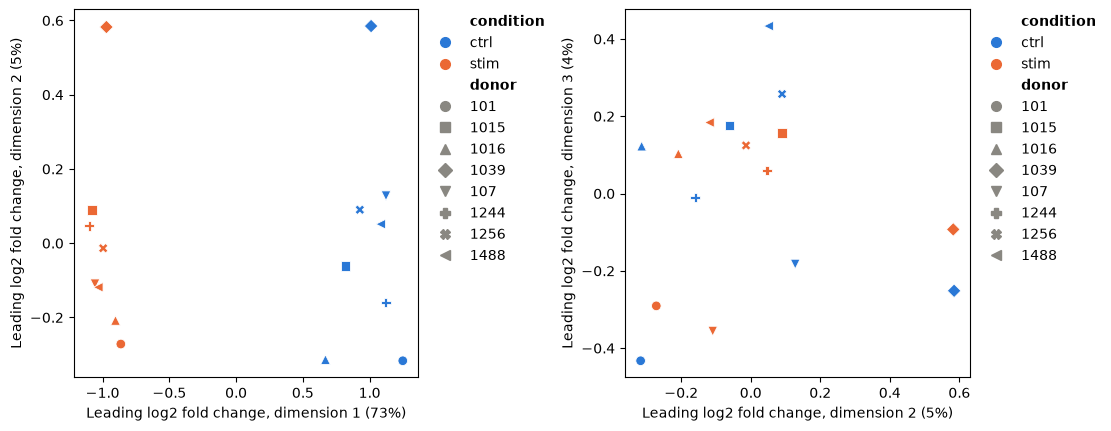
The first dimension, nearly three quarters of the variation, is the stimulation. The next ones are the donors: the two samples of each donor lie near each other, and donor 1039 stands apart from the rest. Differences between donors are why the design pairs each donor’s samples (Genes that change in each cell type). A sample far from its group on such a plot deserves a look before any test.
Which genes to test
voom estimates how the variance of the log counts falls with their level, and weights
every observation by it Law et al., 2014; its plot (plot_mean_variance) shows the
trend. Genes whose counts are mostly zeros have log-CPM
values near the floor in most samples: their spread is small for want of counts, not
because they are precise, and they bend the trend down at its low end, where voom
would then weight noisy observations most. filter_by_expression keeps the
genes with enough counts in enough samples, edgeR’s filterByExpr rule Chen et al., 2016,
and the number of samples it asks for comes from the design.
design = Design(
    kang.samples,
    "~ donor + condition",
    levels={"condition": ["ctrl", "stim"]},
    contrasts={"stim_vs_ctrl": "conditionstim"},
)
counts = kang.layer("counts", "CD14+ Monocytes")
detected = np.count_nonzero(counts, axis=0) >= 2
keep = filter_by_expression(counts, design=design)
by_condition = filter_by_expression(counts, group=kang.samples["condition"])
print(f"{detected.sum():>6,} genes with counts in at least two samples")
print(f"{keep.sum():>6,} kept by the filter with the paired design")
print(f"{by_condition.sum():>6,} kept by the filter with the condition as the group")

figure, (left, right) = plt.subplots(
    1, 2, figsize=(11, 4), layout="constrained", sharey=True
)
for ax, genes, title in (
    (left, detected, "Genes with counts in two samples"),
    (right, keep, "Genes kept by the filter"),
):
    plot_mean_variance(
        voom(counts[:, genes], design, norm_factors=tmm_factors(counts[:, genes])),
        ax=ax,
    )
    ax.set_title(title)
plt.show()
12,966 genes with counts in at least two samples
5,125 kept by the filter with the paired design
3,651 kept by the filter with the condition as the group
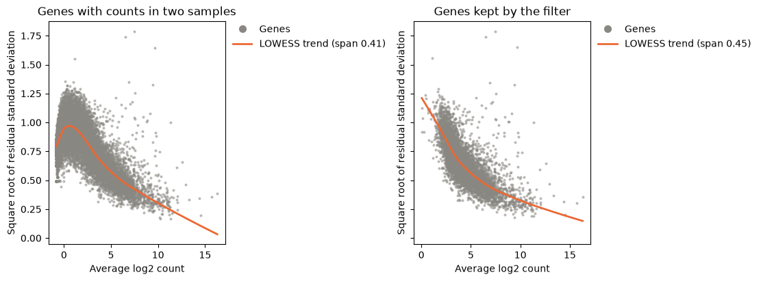
Without the filter, the trend falls at the low end, as the genes with mostly zero counts pull it down; with it, the trend falls steadily with the expression level, the shape voom expects. The number of samples a gene needs comes from the design’s largest leverage: with the paired design, every sample’s profile has a leverage of 9/16, so a gene needs enough counts in two samples; with the condition as the group, in eight, which keeps fewer genes.
Normalization factors
Library sizes account for sequencing depth, not for composition: when a few genes take
a larger share of a library, every other gene looks lower in it. TMM factors
(tmm_factors) rescale the libraries so that most genes do not change between
samples Robinson & Oshlack, 2010, and Count models describes
the alternatives.
stimulated = np.asarray(kang.samples["condition"]) == "stim"
cpm = counts / counts.sum(axis=1, keepdims=True)
gain = cpm[stimulated].mean(axis=0) - cpm[~stimulated].mean(axis=0)
rising = np.argsort(gain)[-20:]
print(
    "The 20 genes that gain most take "
    f"{cpm[~stimulated][:, rising].sum(axis=1).mean():.0%} of the control libraries "
    f"and {cpm[stimulated][:, rising].sum(axis=1).mean():.0%} of the stimulated ones.\n"
)

kept = counts[:, keep]
library_sizes = kept.sum(axis=1)
deseq2 = median_ratio_size_factors(kept) / library_sizes
factors = {
    "TMM": tmm_factors(kept),
    "RLE": rle_factors(kept),
    "upper quartile": upper_quartile_factors(kept),
    "DESeq2": deseq2 / np.exp(np.mean(np.log(deseq2))),
}
print(f"{'median factor':<16}{'control':>9}{'stimulated':>12}")
for name, values in factors.items():
    print(
        f"{name:<16}{np.median(values[~stimulated]):>9.2f}"
        f"{np.median(values[stimulated]):>12.2f}"
    )
The 20 genes that gain most take 4% of the control libraries and 22% of the stimulated ones.
median factor control stimulated
TMM 1.19 0.83
RLE 1.19 0.84
upper quartile 1.06 0.93
DESeq2 1.19 0.84
Twenty genes that the stimulation raises take a fifth of the stimulated monocytes’ reads, and the factors correct for it: TMM, RLE and DESeq2’s size factors agree that the stimulated libraries count for about 0.83 of their size and the control ones about 1.19, so that without them most genes would look lower after the stimulation. The upper quartile, which scales each library by one quantile of its counts, corrects less.
Genes with outlying variances
After voom, the residual variances of the genes should not depend on their expression,
and empirical Bayes moderation shrinks each towards a common prior
(Empirical Bayes moderation). limma’s plotSA
(plot_residual_variances) shows them, and robust=True estimates the prior so
that genes with outlying variances do not distort it Phipson et al., 2016.
weights = voom(kept, design, norm_factors=tmm_factors(kept))
fit = contrasts_fit(
    fit_linear_model(weights.log_cpm, design, weights=weights.weights),
    design.contrasts,
)
plain, robust = moderated_statistics(fit), moderated_statistics(fit, robust=True)
symbols = np.asarray(kang.features["symbol"])[keep]
print(
    f"prior degrees of freedom: {plain.prior_df:.1f}, robust {np.max(robust.prior_df):.1f}"
)
print(
    "largest residual variances:", ", ".join(symbols[np.argsort(fit.sigma)[-12:][::-1]])
)
plot_residual_variances(robust)
plt.show()
prior degrees of freedom: 11.4, robust 27.7
largest residual variances: HBB, HBA2, HBA1, ISG15, CCL3, IFITM3, CCL2, CCL4, APOBEC3A, CXCL10, IFI6, LY6E
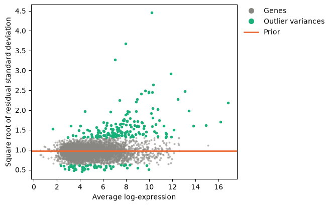
The genes with the largest variances are those of hemoglobin, whose reads come from red cells that contaminate some samples more than others, and interferon-stimulated genes and chemokines whose response differs between donors; the plot marks 217 outlying variances. Robust moderation gives such genes smaller prior degrees of freedom, so that their variances stay closer to their own estimates, and raises those of the other genes from 11.4 to 27.7, whose variances are then shrunk more, which gives their tests more power.
A sample of poor quality
A sample that follows the model less closely than the others, such as a degraded one,
adds noise to every gene. Sample quality weights estimate how closely each sample
follows the model and down-weight it, instead of removing it Liu et al., 2015; Precision
weights gives the model. In the simulated bulk
experiment, sample drug_b_3 has four times the dispersion of the others.
bulk = read_cube("simulated_bulk.cube.zarr")
truth = np.load("simulated_bulk_truth.npz")
bulk_design = Design(
    bulk.samples,
    "~ batch + condition",
    levels={"condition": ["control", "drug_a", "drug_b"]},
    contrasts={"drug_b_vs_control": "conditiondrug_b"},
)
equal = limma_voom(bulk, bulk_design)
weighted = limma_voom(bulk, bulk_design, quality_weights=True)

figure, (left, right) = plt.subplots(1, 2, figsize=(11, 4.2), layout="constrained")
plot_mds(bulk, color_by="condition", marker_by="batch", labels=True, ax=left)
plot_sample_weights(weighted, ax=right)
plt.show()

changed = set(bulk.features["feature_id"][truth["true_log2_fold_change_drug_b"] != 0])
for name, result in (("equal weights", equal), ("quality weights", weighted)):
    table = result.table("bulk", "drug_b_vs_control")
    called = table["feature_id"][table["adjusted_p_value"] < 0.05]
    true = sum(gene in changed for gene in called)
    print(f"{name:<16} {called.size} genes called, {called.size - true} of them false")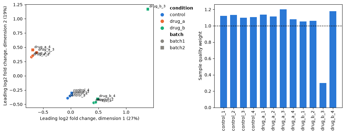
equal weights    192 genes called, 11 of them false
quality weights  204 genes called, 12 of them false
The noisy sample stands apart on the MDS plot and gets a weight of 0.30, while the others weigh slightly more than one, as the weights multiply to one. Down-weighting it finds more of the genes that drug B changes, with about the same number of false calls.
Check the design
A label typed differently in one sample splits a group in two, and the analysis then
runs without an error. Design.check reports such problems, with what to do;
here one stimulated sample is labelled Stim.
labels = list(kang.samples["condition"])
labels[5] = "Stim"
mislabelled = kang.samples.with_columns(condition=labels)
print(Design(mislabelled, "~ donor + condition").check())
Design check: 16 samples, 10 columns, rank 10, 6 residual degrees of freedom.
3 warnings:
1. [similar_levels] condition has levels that differ only in case or surrounding
spaces ('Stim' and 'stim'), and each is a group of its own; if they mean the same
group, clean the labels before building the design
2. [single_sample_level] condition has a single sample at level 'Stim' (1016_stim);
effects of such a level rest on one sample with no replicate. Add replicates, merge
the level with a similar one, or remove the sample
3. [unreplicated_sample] the model fits sample 1016_ctrl (donor = 1016, condition =
ctrl) exactly (leverage 1), so it tells nothing about the residual variance and the
effects it determines rest on it alone. This happens when a level, or a combination
of levels in an interaction, has too few samples for the terms that involve it; add
replicates or simplify the formula
The check also finds aliased and confounded columns, levels without samples, contrasts the design cannot estimate and numeric codes that look like batches (Designs, linear models and contrasts).
Choices
The filter.
limma_voomfilters with the design, as above; a paired design gives every sample a high leverage, so a gene needs counts in only a few samples.expression_filterchanges the thresholds, andfilter_by_expressionwithgroup=asks for counts in as many samples as the smallest group has.Normalization factors. TMM is the default of
limma_voomand of edgeR. TMM, RLE and DESeq2’s median ratios assume that most genes do not change between samples, and the upper quartile that one quantile of the counts does not; when a response changes many genes, check that the factors make sense, as above.Robust moderation. Pass
robust=Truetolimma_voomwhenplotSAshows outlying variances, as here.A poor sample. Quality weights keep it at a lower weight; leaving it out loses its information, and in a paired design its partner’s (Precision weights).
prior_weights="n_cells"instead weights pseudobulk profiles by their number of cells; the two cannot be combined.What to adjust for. Repeated measures and donors partitions the variance of every gene among the variables of the design.
- Kang, H. M., Subramaniam, M., Targ, S., Nguyen, M., Maliskova, L., McCarthy, E., Wan, E., Wong, S., Byrnes, L., Lanata, C. M., Gate, R. E., Mostafavi, S., Marson, A., Zaitlen, N., Criswell, L. A., & Ye, C. J. (2018). Multiplexed droplet single-cell RNA-sequencing using natural genetic variation. Nature Biotechnology, 36(1), 89–94. 10.1038/nbt.4042
- Law, C. W., Chen, Y., Shi, W., & Smyth, G. K. (2014). voom: precision weights unlock linear model analysis tools for RNA-seq read counts. Genome Biology, 15(2), R29. 10.1186/gb-2014-15-2-r29
- Chen, Y., Lun, A. T. L., & Smyth, G. K. (2016). From reads to genes to pathways: differential expression analysis of RNA-Seq experiments using Rsubread and the edgeR quasi-likelihood pipeline. F1000Research, 5, 1438. 10.12688/f1000research.8987.2
- Robinson, M. D., & Oshlack, A. (2010). A scaling normalization method for differential expression analysis of RNA-seq data. Genome Biology, 11(3), R25. 10.1186/gb-2010-11-3-r25
- Phipson, B., Lee, S., Majewski, I. J., Alexander, W. S., & Smyth, G. K. (2016). Robust hyperparameter estimation protects against hypervariable genes and improves power to detect differential expression. The Annals of Applied Statistics, 10(2), 946–963. 10.1214/16-AOAS920
- Liu, R., Holik, A. Z., Su, S., Jansz, N., Chen, K., Leong, H. S., Blewitt, M. E., Asselin-Labat, M.-L., Smyth, G. K., & Ritchie, M. E. (2015). Why weight? Modelling sample and observational level variability improves power in RNA-seq analyses. Nucleic Acids Research, 43(15), e97. 10.1093/nar/gkv412