Repeated measures and donors

When a study samples each donor more than once, before and after a treatment, at several time points or in several tissues, the samples of a donor are correlated. Two models allow for it: a fixed effect for each donor, which compares each donor’s samples with each other, and a random effect for the donor, which dream fits by a mixed model for every gene Hoffman & Roussos, 2021. This page compares the two on the Kang data Kang et al., 2018, tests a variable of the donors and several time points on a simulated study whose truth is known, and measures how much of each gene’s variation the donors explain. Mixed models, REML and dream explains the models.

A fixed or a random donor effect¶

In the Kang data every donor gives one control and one stimulated sample. The paired design ~ donor + condition and the mixed model ~ condition with (1 | donor) both compare the stimulated samples with the controls of the same donors.

import matplotlib.pyplot as plt
import numpy as np

import cytepool
from cytepool.cube import Cube
from cytepool.design import Design
from cytepool.differential_expression import dream_voom, limma_voom
from cytepool.io import read_cube
from cytepool.plotting import (
    plot_gene_variance_fractions,
    plot_p_values,
    plot_variance_fractions,
)
from cytepool.variance_partitioning import variance_partitioning

kang = read_cube("kang2018.cube.zarr")
print(f"CytePool {cytepool.__version__}")
monocytes = "CD14+ Monocytes"
levels = {"condition": ["ctrl", "stim"]}
contrasts = {"stim_vs_ctrl": "conditionstim"}
paired = Design(kang.samples, "~ donor + condition", levels=levels, contrasts=contrasts)
mixed = Design(
    kang.samples,
    "~ condition",
    random="(1 | donor)",
    levels=levels,
    contrasts=contrasts,
)
fixed = limma_voom(kang, paired, groups=monocytes).table(monocytes, "stim_vs_ctrl")
random = dream_voom(kang, mixed, groups=monocytes).table(monocytes, "stim_vs_ctrl")

for name, table in (("fixed donor effect", fixed), ("random donor effect", random)):
    called = np.count_nonzero(table["adjusted_p_value"] < 0.05)
    print(f"{name:<20} {table['feature_id'].size:>6,} genes tested {called:>6,} called")
shared, i, j = np.intersect1d(
    fixed["feature_id"], random["feature_id"], return_indices=True
)
correlation = np.corrcoef(fixed["log2_fold_change"][i], random["log2_fold_change"][j])
both = (fixed["adjusted_p_value"][i] < 0.05) & (random["adjusted_p_value"][j] < 0.05)
print(
    f"Of the {shared.size:,} genes both test, the log2 fold changes correlate at "
    f"{correlation[0, 1]:.3f} and {both.sum():,} are called by both."
)

CytePool 0.1.dev54+g3f0cbb52e

fixed donor effect    5,125 genes tested  3,168 called
random donor effect   3,651 genes tested  2,542 called
Of the 3,651 genes both test, the log2 fold changes correlate at 0.999 and 2,273 are called by both.

Both models find the same response: the fold changes of the genes both test agree almost exactly, and most genes that one calls the other calls too. They test different numbers of genes because each filters with its own fixed effects, and the paired design asks for counts in fewer samples than the condition alone (Normalization, filtering and sample quality). When every donor gives a sample in every condition and the question is within donors, the paired design is the simpler of the two.

A variable of the donors¶

A study of patients and healthy donors, each sampled at three time points, asks two kinds of question: what changes over time within donors, and how patients differ from healthy donors. The simulation below has three patients and three healthy donors, each sampled at 0, 6 and 24 hours, in one cell type: time changes 400 of 4,000 genes, the disease 150 others, and every donor shifts every gene a little in all its samples. A paired design cannot hold the disease, which is constant within each donor, and Design.check says why.

rng = np.random.default_rng(20261026)
n_genes, times = 4_000, ["0h", "6h", "24h"]
donors = ["P1", "P2", "P3", "H1", "H2", "H3"]
genes = np.array([f"gene_{g:04d}" for g in range(1, n_genes + 1)])
baseline = rng.normal(0.0, 1.5, n_genes)
dispersion = 0.05 * rng.lognormal(0.0, 0.5, n_genes)
donor_spread = 0.35 * rng.lognormal(0.0, 0.4, n_genes)
time_effect = {time: np.zeros(n_genes) for time in times}
changed = rng.choice(n_genes, 400, replace=False)
for time, chosen in (("6h", changed[:250]), ("24h", changed[150:])):
    time_effect[time][chosen] = rng.choice([-1, 1], 250) * rng.uniform(0.6, 1.8, 250)
disease_effect = np.zeros(n_genes)
in_disease = rng.choice(np.setdiff1d(np.arange(n_genes), changed), 150, replace=False)
disease_effect[in_disease] = rng.choice([-1, 1], 150) * rng.uniform(0.8, 2.0, 150)

rows, counts = [], []
for donor in donors:
    shift = rng.normal(0.0, donor_spread)  # the donor's own level of every gene
    patient = donor.startswith("P")
    for time in times:
        log2_mean = baseline + shift + time_effect[time] + patient * disease_effect
        mean = rng.uniform(1e6, 4e6) * 2.0**log2_mean / np.sum(2.0**log2_mean)
        counts.append(rng.poisson(rng.gamma(1 / dispersion, mean * dispersion)))
        rows.append(
            (f"{donor}_{time}", donor, "patient" if patient else "healthy", time)
        )
samples = dict(zip(("sample_id", "donor", "disease", "time"), map(list, zip(*rows))))
study = Cube(
    {"counts": np.array(counts, dtype=np.uint32)[np.newaxis]},
    samples=samples,
    groups={"group_id": ["Monocytes"]},
    features={"feature_id": genes},
)
print(Design(study.samples, "~ donor + disease + time").check())

Design check: 18 samples, 9 columns, rank 8, 10 residual degrees of freedom.
2 errors:
  1. [rank_deficient] the design matrix has 9 columns but rank 8, so 1 coefficient is
     not estimable. Aliased columns: diseasepatient = donorP1 + donorP2 + donorP3. The
     columns in each relation cannot be estimated separately; remove or recode the
     variables behind them (see the other findings), or drop terms from the formula
  2. [confounded] every level of donor holds a single level of disease (disease
     'healthy': donor 'H1', 'H2' and 'H3'; disease 'patient': donor 'P1', 'P2' and
     'P3'), so the effect of disease cannot be separated from the donor effects. Remove
     donor from the formula; if donor groups repeated samples (donors, batches), the
     right model has it as a random effect, random='(1 | donor)'; fit_mixed_model
     estimates this random intercept by REML; fit_linear_model fits it with a known
     correlation, given block= (the donor of each sample) and correlation=; or pool the
     samples of each donor with Cube.collapse_samples('donor')

The random donor effect keeps the disease testable. dream_voom tests each contrast, and f_tests tests several at once: here whether a gene changes at any time point, by one F-test instead of a test per time point. With fewer than 20 samples it uses Kenward and Roger’s degrees of freedom, which allow for variance components estimated from few donors Kenward & Roger, 1997. The simulation knows which genes changed.

levels = {"disease": ["healthy", "patient"], "time": times}
design = Design(
    study.samples,
    "~ disease + time",
    random="(1 | donor)",
    levels=levels,
    contrasts={
        "patient_vs_healthy": "diseasepatient",
        "6h_vs_0h": "time6h",
        "24h_vs_0h": "time24h",
    },
)
result = dream_voom(study, design, f_tests={"time": ["6h_vs_0h", "24h_vs_0h"]})
print("degrees of freedom:", result.summary["df_method"][0], "\n")

truth = {
    "patient_vs_healthy": disease_effect != 0,
    "6h_vs_0h": time_effect["6h"] != 0,
    "24h_vs_0h": time_effect["24h"] != 0,
    "time (F-test)": (time_effect["6h"] != 0) | (time_effect["24h"] != 0),
}
print(f"{'test':<20}{'changed':>8}{'called':>8}{'false':>7}")
for name, true_change in truth.items():
    table = result.table("Monocytes", name.removesuffix(" (F-test)"))
    effect = true_change[np.searchsorted(genes, table["feature_id"])]
    called = table["adjusted_p_value"] < 0.05
    print(f"{name:<20}{effect.sum():>8}{called.sum():>8}{(called & ~effect).sum():>7}")

degrees of freedom: kenward_roger 

test                 changed  called  false
patient_vs_healthy       150     109     28
6h_vs_0h                 250     232     14
24h_vs_0h                250     218      4
time (F-test)            400     387     18

The tests within donors find most of the genes that time changes, with few false calls. The test between donors does not hold its error rate: 28 of its 109 calls are false, where an adjustment at 5% allows for about 5 on average. With three donors in each group, a difference between patients and healthy donors is measured against the variation between six donors, which every gene’s model estimates from those six alone. The p-values of the 3,850 genes that the disease leaves unchanged should be uniform. Pooling each donor’s samples into one profile (Cube.collapse_samples) gives six profiles, whose residuals hold the variation between donors, and limma_voom compares them.

pooled = study.collapse_samples("donor")
pooled_design = Design(
    pooled.samples,
    "~ disease",
    levels={"disease": ["healthy", "patient"]},
    contrasts={"patient_vs_healthy": "diseasepatient"},
)
by_donor = limma_voom(pooled, pooled_design)

figure, (left, right) = plt.subplots(
    1, 2, figsize=(11, 3.8), layout="constrained", sharey=True
)
for ax, tested, title in (
    (left, result, "dream_voom, every sample"),
    (right, by_donor, "limma_voom, samples pooled by donor"),
):
    table = tested.table("Monocytes", "patient_vs_healthy")
    unchanged = disease_effect[np.searchsorted(genes, table["feature_id"])] == 0
    plot_p_values(table["p_value"][unchanged], ax=ax)
    ax.set_title(title)
    called = table["adjusted_p_value"] < 0.05
    print(
        f"{title}: {called.sum()} genes called, {(called & unchanged).sum()} of them false"
    )
plt.show()

dream_voom, every sample: 109 genes called, 28 of them false
limma_voom, samples pooled by donor: 62 genes called, 3 of them false

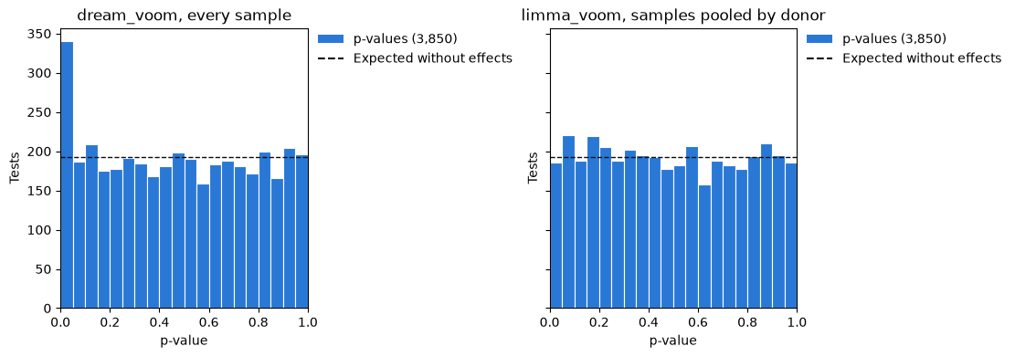
Two histograms of the p-values of the 3,850 genes that the simulated disease leaves unchanged, in 20 bins of width 0.05, each with a dashed line at the count expected without effects, about 193. Left, dream_voom on every sample: the first bin, p-values below 0.05, holds about 340 genes, and the other bins about the expected count. Right, limma_voom on the profiles pooled by donor: every bin holds close to the expected count.

dream_voom’s p-values of the unchanged genes gather below 0.05, about 1.8 times as many as expected there; those of the pooled profiles are uniform, and 3 of their 62 calls are false. The pooled comparison finds fewer genes, but those it finds hold. Pooling suits a design in which every donor was sampled alike, as here; the changes within donors are tested on every sample, where dream_voom kept their error rate.

What drives the variation between samples¶

Variance partitioning fits every gene with a mixed model of every variable of the design and reports the share of its variance that each explains Hoffman & Schadt, 2016, as variancePartition does. It shows which variables dominate, and which genes follow each. variance_partitioning runs it on every cell type of a cube, after the same steps as dream_voom.

partition_design = Design(
    kang.samples, "~ 1", random=["(1 | donor)", "(1 | condition)"]
)
partition = variance_partitioning(kang, partition_design, groups=monocytes)
chosen = ["ISG15", "CD14", "S100A8", "RPS26", "HBB", "HLA-DQA1", "HLA-DRA", "LYZ"]

fractions = partition.table(monocytes)
shares = [f"{name} {np.median(fractions[name]):.0%}" for name in partition.variables]
print("median share of a gene's variance:", ", ".join(shares))

figure, (left, right) = plt.subplots(1, 2, figsize=(11, 4.5), layout="constrained")
plot_variance_fractions(partition, ax=left)
plot_gene_variance_fractions(partition, chosen, ax=right)
plt.show()

median share of a gene's variance:

 donor 8%, condition 43%, residuals 34%

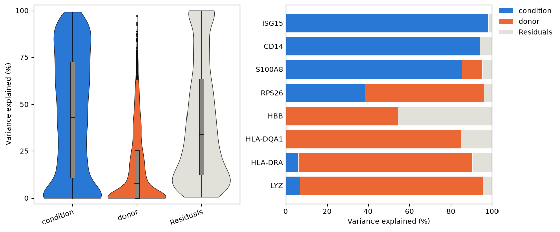
Two panels of variance partitioning in the CD14+ monocytes. Left, violins of the percentage of each gene's variance that the condition, the donor and the residuals explain, with a narrow box plot inside each: the condition spreads from 0 to 100% with a median near 43%, the donor lies mostly below 25% with a median near 8% and a tail of genes up to 97%, and the residuals spread from 0 to 100% with a median near 34%. Right, stacked bars for eight genes: ISG15, CD14 and S100A8 are mostly condition; RPS26 is about 38% condition and 58% donor; HBB about 54% donor and 46% residuals; HLA-DQA1, HLA-DRA and LYZ are mostly donor.

The stimulation explains much of the variance of most genes, and the donors a little of most, but the genes differ widely. ISG15 and CD14 vary almost only with the stimulation; the HLA class II genes HLA-DQA1 and HLA-DRA, which differ between people, and LYZ vary mostly between donors, and RPS26 with both. HBB, whose reads come from contaminating red cells, varies between donors and between the two samples of each donor, which the residuals hold.

Choices¶

A fixed or a random donor effect. With every donor in every condition and a question within donors, the paired design and limma_voom are the simplest. A variable of the donors, such as disease, sex or age, needs the random effect and dream_voom, and so do donors with unequal numbers of samples.
Few donors, a question between donors. With three donors in each group, dream_voom’s test between donors called too many genes above. When every donor was sampled alike, compare the profiles pooled by donor (Cube.collapse_samples) with limma_voom instead, and test the changes within donors with dream_voom.
Degrees of freedom. df_method="adaptive", the default, uses Kenward and Roger’s below 20 samples and Satterthwaite’s from 20; "kenward_roger" and "satterthwaite" fix one (Mixed models, REML and dream).
Several time points or groups. f_tests asks whether anything changes among them; the contrasts then say what changes when.
What to adjust for. A variable that explains much of the variance of many genes and is not the question, such as a batch, is worth a term in the design. Normalization, filtering and sample quality shows how to look for outlying samples.

References¶

Hoffman, G. E., & Roussos, P. (2021). Dream: powerful differential expression analysis for repeated measures designs. Bioinformatics, 37(2), 192–201. 10.1093/bioinformatics/btaa687
Kang, H. M., Subramaniam, M., Targ, S., Nguyen, M., Maliskova, L., McCarthy, E., Wan, E., Wong, S., Byrnes, L., Lanata, C. M., Gate, R. E., Mostafavi, S., Marson, A., Zaitlen, N., Criswell, L. A., & Ye, C. J. (2018). Multiplexed droplet single-cell RNA-sequencing using natural genetic variation. Nature Biotechnology, 36(1), 89–94. 10.1038/nbt.4042
Kenward, M. G., & Roger, J. H. (1997). Small sample inference for fixed effects from restricted maximum likelihood. Biometrics, 53(3), 983–997. 10.2307/2533558
Hoffman, G. E., & Schadt, E. E. (2016). variancePartition: interpreting drivers of variation in complex gene expression studies. BMC Bioinformatics, 17(1), 483. 10.1186/s12859-016-1323-z