Find which genes respond to a dose in each cell type of a dose series, how, and from which dose, with dose_response, and check the calls against noise with permutation_check. The series here is simulated from known curves by simulate_dose_series, so its truth says which genes respond: 27 mice, 3 for the vehicle and for each of eight doses from 0.01 to 30 ug/kg in half-log steps, with hepatocytes, macrophages, stellate cells and cholangiocytes, of which 20%, 15%, 5% and 10% of 2,000 genes respond. Hepatocytes and stellate cells fall by half and macrophages double at the top dose, and cholangiocytes are rare. Dose response explains the methods.
import json
from collections import Counter
from pathlib import Path

import matplotlib.pyplot as plt
import numpy as np

import cytepool
from cytepool import (
    CandidateShapes,
    Design,
    DoseAxis,
    DoseTruth,
    dose_response,
    permutation_check,
    read_cube,
)
from cytepool.plotting import plot_dose_response

# The cube, and the truth of each cell type.
cube = read_cube("simulated_dose_series.cube.zarr")
truth = DoseTruth(**json.loads(Path("simulated_dose_series_truth.json").read_text()))
print(f"CytePool {cytepool.__version__}")
print(cube)
CytePool 0.1.1.dev19+gb33f62f82
Cube with 27 samples x 4 groups x 2,000 features
layers: counts (uint32, lazy)
filled: 108 of 108 sample x group entries have cells (100.0%)
samples: sample_id, dose, dose_group, donor
groups: group_id
features: feature_id
Each sample is one mouse’s pseudobulk profile in one cell type: the sum of its cells’ counts. The sample table holds each mouse’s dose, 0 for the vehicle.
Place the doses on an axis
Where does each dose sit on the curve’s axis? The doses are spaced by half a log10, so the curves follow log10 dose, and the vehicle, whose dose of 0 has no logarithm, forms a group of its own, the default of DoseAxis:
axis = DoseAxis("dose", unit=truth.unit, metric=truth.metric)
print(axis)
DoseAxis(column='dose', unit='ug/kg', metric='administered', scale='log10', vehicle='own_group', offset=None)
Test every cell type
Which genes respond in each cell type? dose_response takes the design of the terms other than dose, here none ("~ 1"). It checks the design first, as check_dose_design does, so that check needs no call of its own, and tests the cell types that support tests:
result = dose_response(cube, Design(cube.samples, "~ 1"), dose=axis)
print(result)
DoseResponseResult (limma_voom): 4 cell types, 3 tested; tests: spline,
nonlinearity, linear_trend, dose_groups
dose: ug/kg (administered) on a log10 axis, the vehicle in a group of its own;
spline of 2 columns, knots at 0.548 ug/kg, boundary knots at 0.01 and 30
ug/kg; linear_trend slopes per log10 unit of dose
gate: spline test, Benjamini-Hochberg within each cell type, at 5% FDR
Hepatocyte: 9 dose groups, 27 samples, 1,869 genes; 230 pass the gate; calls
at 5% FDR: spline 230, nonlinearity 98, linear_trend 205,
dose_groups 201
Macrophage: 9 dose groups, 27 samples, 1,484 genes; 113 pass the gate; calls
at 5% FDR: spline 113, nonlinearity 41, linear_trend 94,
dose_groups 104
Stellate: 9 dose groups, 27 samples, 845 genes; 17 pass the gate; calls at 5%
FDR: spline 17, nonlinearity 3, linear_trend 12, dose_groups 10
Cholangiocyte: not tested, descriptive: no treated dose group that can be
compared with the vehicle keeps a second sample, so no dose has
a replicate
The printout gives the spline’s knot in doses, the gate, which decides which genes count as responding, and, for each cell type, the dose groups it compares, its samples and genes, the genes that pass the gate and the genes each test calls at 5% FDR. Read spline first, the default gate: it asks whether a gene responds at all. linear_trend and nonlinearity describe the responses it finds, and dose_groups asks the same question as spline without a curve. The cholangiocytes are not tested: few of their profiles keep 10 cells, so no dose has a second replicate, and the check calls them descriptive. Its report stays in the result:
report = result.design_report
report.doses.filter(group_id="Cholangiocyte").select(
    ["dose", "n_samples_used", "n_cells_min"]
)
Table with 9 rows and 3 columns
dose n_samples_used n_cells_min
float64 int64 float64
0.0 1 17.0
0.01 0 nan
0.03 1 13.0
0.1 0 nan
0.3 1 10.0
1.0 1 11.0
3.0 0 nan
10.0 1 14.0
30.0 1 13.0Read a test’s table
What does each gene’s row say? The table of a test has one row per gene that passes the expression filter, here the first five rows of the hepatocytes’ spline, sorted by p-value:
# The table of the hepatocytes' spline test, and its five genes of smallest p-value.
spline = result.table("Hepatocyte", "spline")
top = spline.sort("p_value").take(range(5))
print(
    f"{'feature_id':<12}{'f_statistic':>12}{'p_value':>10}{'adjusted_p_value':>18}"
    f"{'adjusted_p_value_across_groups':>32}"
)
for gene, f_statistic, p_value, adjusted, across in zip(
    top["feature_id"],
    top["f_statistic"],
    top["p_value"],
    top["adjusted_p_value"],
    top["adjusted_p_value_across_groups"],
):
    print(
        f"{gene:<12}{f_statistic:>12.1f}{p_value:>10.2g}{adjusted:>18.2g}{across:>32.2g}"
    )
feature_id f_statistic p_value adjusted_p_value adjusted_p_value_across_groups
gene_0295 163.6 4.5e-19 3.2e-16 3.6e-16
gene_0896 163.6 4.5e-19 3.2e-16 3.6e-16
gene_0046 162.1 5.1e-19 3.2e-16 3.6e-16
gene_0342 111.4 1.1e-16 5.2e-14 5.2e-14
gene_0708 98.4 6.4e-16 2.4e-13 2.7e-13
f_statistic and p_value test the gene; adjusted_p_value adjusts the p-values of the cell type by Benjamini-Hochberg, and adjusted_p_value_across_groups those of every cell type at once. The table of the linear trend, result.table("Hepatocyte", "linear_trend"), has a log2_fold_change, the slope of a straight line along the axis, the change per log10 unit of dose, and result.table("Hepatocyte", "each_dose") tests each dose against the vehicle.
Compare the calls with the truth
How many of the genes that respond does each test find, and how many flat genes does it call? The truth knows each gene’s maximal change:
for cell_type in ("Hepatocyte", "Macrophage", "Stellate"):
    genes = truth.table(cell_type)
    change = dict(
        zip(genes["feature_id"].tolist(), np.abs(genes["max_log2_change"]).tolist())
    )
    for test in result.tests:
        table = result.table(cell_type, test)
        called = np.asarray(table["adjusted_p_value"]) <= 0.05
        responds = np.array([change[g] > 0 for g in table["feature_id"].tolist()])
        print(
            f"{cell_type:<11} {test:<13} {called[responds].sum():>3} of "
            f"{responds.sum()} responsive genes, {called[~responds].sum()} of "
            f"{(~responds).sum()} flat"
        )
Hepatocyte spline 222 of 378 responsive genes, 8 of 1491 flat
Hepatocyte nonlinearity 93 of 378 responsive genes, 5 of 1491 flat
Hepatocyte linear_trend 194 of 378 responsive genes, 11 of 1491 flat
Hepatocyte dose_groups 194 of 378 responsive genes, 7 of 1491 flat
Macrophage spline 109 of 223 responsive genes, 4 of 1261 flat
Macrophage nonlinearity 40 of 223 responsive genes, 1 of 1261 flat
Macrophage linear_trend 90 of 223 responsive genes, 4 of 1261 flat
Macrophage dose_groups 100 of 223 responsive genes, 4 of 1261 flat
Stellate spline 17 of 49 responsive genes, 0 of 796 flat
Stellate nonlinearity 3 of 49 responsive genes, 0 of 796 flat
Stellate linear_trend 12 of 49 responsive genes, 0 of 796 flat
Stellate dose_groups 10 of 49 responsive genes, 0 of 796 flat
With three mice per dose, the spline finds about 6 in 10 of the hepatocytes’ responses and calls 8 of their 1,491 flat genes. The stellate cells, with 40 cells per profile, give noisier profiles, and their spline finds about a third of their responses. The non-linearity test calls fewer genes: only the responses that bend away from a straight line along log10 dose, such as bells and steps.
See the shape of a response
What shape does a response take? plot_dose_response draws each dose’s estimate against the vehicle, the fitted spline and its 95% band; the true curves are drawn dashed over them:
called = spline.filter(spline["adjusted_p_value"] <= 0.05)
truths = truth.table("Hepatocyte")
shape_of = dict(zip(truths["feature_id"].tolist(), truths["shape"].tolist()))
# The gene of smallest p-value of each of four shapes.
ordered = called.sort("p_value")["feature_id"].tolist()
shapes = ("hill", "log_gauss_probit", "step", "linear")
picked = [next(g for g in ordered if shape_of[g] == shape) for shape in shapes]
ax = plot_dose_response(result, "Hepatocyte", genes=picked)
# The true curves, dashed, in the colours of the fitted ones.
grid = np.geomspace(0.01, 30.0, 100)
true = truth.curve("Hepatocyte", picked, at=grid)
fitted = [line for line in ax.get_lines() if line.get_gid() == "curve"]
for line, values in zip(fitted, true, strict=True):
    ax.plot(axis.positions(grid), values, linestyle="--", color=line.get_color())
plt.show()
print(", ".join(f"{g}: {shape_of[g]}" for g in picked))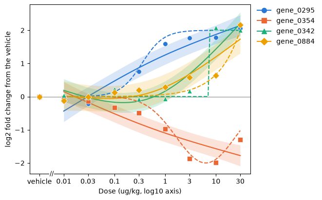
gene_0295: hill, gene_0354: log_gauss_probit, gene_0342: step, gene_0884: linear
A spline of two columns follows its gene’s dose groups only as far as its shape allows. The Hill gene (gene_0295) rises more steeply between 0.3 and 3 ug/kg than its spline, which also starts at -0.4 at 0.01 ug/kg, where the true change is 0; its band misses the true curve at 4 of the 8 doses. The bell (gene_0354) turns back above 10 ug/kg while its spline keeps falling, and its band misses the true curve from 0.1 ug/kg up. The step’s spline (gene_0342) smooths its jump at 7 ug/kg, and the straight line in dose (gene_0884), which climbs only at the top doses, gets a spline that rises earlier; both bands miss at 3 and 10 ug/kg. A band holds the spline that the true means of the dose groups would give, not every true curve, so read it beside the dose points, which lie closer to the truth. With the vehicle in a group of its own, each curve starts at the lowest dose, a jump from the vehicle’s 0 left of the axis break. A larger spline_df follows such shapes more closely at some cost in power, and the non-linearity test flags the responses that bend.
Test a few expected shapes
Does a response follow one of a few expected shapes, or grow with dose? The spline finds responses of any shape. Two multiple contrast tests ask the narrower questions: the MCP step of MCP-Mod (multiple comparison procedure and modelling) tests a few candidate shapes, and the Williams-type test responses that grow in dose order. On 20,000 genes and 7 doses they add 10 to 23 s each to the 0.9 s of the default tests, so they run only when named in tests, here beside the spline. CandidateShapes.spread places the default shapes over the doses, as dose_response does when no candidates are given; each shape’s change is 1 at the top dose, or at its peak:
shapes = CandidateShapes.spread(axis, cube.samples)
# Each shape along the axis's log10 positions, with a tick at each treated dose.
grid = np.geomspace(0.01, 30.0, 200)
doses = np.unique(np.asarray(cube.samples["dose"]))[1:]
fig, ax = plt.subplots(figsize=(6.5, 3.5))
for name, values in zip(shapes.names, shapes.means(grid), strict=True):
    ax.plot(axis.positions(grid), values, label=name)
ax.set_xticks(axis.positions(doses), [f"{d:g}" for d in doses])
ax.set(xlabel="Dose (ug/kg, log10 axis)", ylabel="Change from the vehicle")
ax.legend(frameon=False)
plt.show()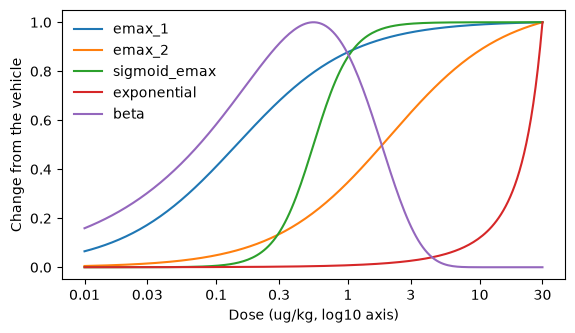
Two Emax shapes rise early and midway along log dose, the sigmoid Emax shape rises steeply midway, the exponential shape rises late, at the top doses, and the beta shape rises to a peak midway and falls back by 10 ug/kg. The two multiple contrast tests run beside the spline:
shaped = dose_response(
    cube,
    Design(cube.samples, "~ 1"),
    dose=axis,
    tests=("spline", "williams", "mcp"),
    rng=1,
)
print(shaped)
DoseResponseResult (limma_voom): 4 cell types, 3 tested; tests: spline,
williams, mcp
dose: ug/kg (administered) on a log10 axis, the vehicle in a group of its own;
spline of 2 columns, knots at 0.548 ug/kg, boundary knots at 0.01 and 30
ug/kg
gate: spline test, Benjamini-Hochberg within each cell type, at 5% FDR
Hepatocyte: 9 dose groups, 27 samples, 1,869 genes; 230 pass the gate; calls
at 5% FDR: spline 230, williams 172, mcp 235
Macrophage: 9 dose groups, 27 samples, 1,484 genes; 113 pass the gate; calls
at 5% FDR: spline 113, williams 92, mcp 121
Stellate: 9 dose groups, 27 samples, 845 genes; 17 pass the gate; calls at 5%
FDR: spline 17, williams 11, mcp 18
Cholangiocyte: not tested, descriptive: no treated dose group that can be
compared with the vehicle keeps a second sample, so no dose has
a replicate
rng seeds the Monte Carlo error of the p-values, so they reproduce. Which responses does each test find, and how many flat genes does it call? Count the calls at 5% FDR by true shape:
genes = truth.table("Hepatocyte")
shape_of = dict(zip(genes["feature_id"].tolist(), genes["shape"].tolist()))
order = [
    "hill",
    "exponential",
    "linear",
    "power",
    "log_gauss_probit",
    "frechet",
    "step",
    "flat",
]
tested = shaped.table("Hepatocyte", "spline")["feature_id"].tolist()
called = {}
for test in ("spline", "williams", "mcp"):
    table = shaped.table("Hepatocyte", test)
    called[test] = set(
        table.filter(table["adjusted_p_value"] <= 0.05)["feature_id"].tolist()
    )
print(f"{'shape':<18}{'genes':>6}{'spline':>8}{'williams':>10}{'mcp':>6}")
for shape in order:
    members = [g for g in tested if shape_of[g] == shape]
    found = [sum(g in called[test] for g in members) for test in called]
    print(f"{shape:<18}{len(members):>6}{found[0]:>8}{found[1]:>10}{found[2]:>6}")
shape genes spline williams mcp
hill 112 56 46 55
exponential 55 29 22 27
linear 20 11 9 13
power 36 17 15 22
log_gauss_probit 77 56 35 54
frechet 39 25 17 25
step 39 28 21 27
flat 1491 8 7 12
The MCP step finds 223 of the 378 responses and the spline 222, and they call 12 and 8 of the 1,491 flat genes; the Williams-type test finds 165 and calls 7. The MCP step and the spline both find most of the 77 bells, the log_gauss_probit curves that rise and fall back, 54 and 56, where the Williams-type test finds 35: it pools the top doses, where a bell has fallen back. Which candidate shape does the MCP step name for the genes it calls?
# The candidate shape of each called gene's largest |t|, by the gene's true shape.
mcp = shaped.table("Hepatocyte", "mcp")
calls = mcp.filter(mcp["adjusted_p_value"] <= 0.05)
for true_shape in ("exponential", "power", "log_gauss_probit"):
    contrasts = Counter(
        contrast
        for gene, contrast in zip(
            calls["feature_id"].tolist(), calls["contrast"].tolist()
        )
        if shape_of[gene] == true_shape
    )
    print(
        f"{true_shape:<17} " + ", ".join(f"{n} {k}" for n, k in contrasts.most_common())
    )
exponential emax_1 16, emax_2 10, exponential 1
power exponential 21, emax_2 1
log_gauss_probit beta 17, sigmoid_emax 14, emax_2 14, emax_1 7, exponential 2
Of the 27 exponential curves the MCP step calls, 26 have an Emax shape as their strongest contrast, and 21 of the 22 power curves the candidate exponential shape: the simulator’s exponential curves, BMDS’s exponential 4, level off as the Emax shapes do, while the candidate exponential shape, BMDS’s exponential 2, rises late, as power curves do. The beta shape is the strongest contrast for 17 of the 54 bells, and Emax or sigmoid Emax shapes for most of the others, since many bells turn back only at the top doses, where they look monotone. So contrast names the candidate whose contrast best matches a gene’s observed changes, not the gene’s shape: the shapes’ contrasts are strongly correlated, and fitting and choosing a shape is MCP-Mod’s modelling step, not implemented yet.
Choose which genes count as responding
Which genes count as responding to the dose? Each test calls its own genes, and one decides: the gate, the spline test at 5% FDR by default, as the printout’s gate line says. Its table gives each gene’s call in passes_gate:
gate = result.table("Hepatocyte", "gate")
print(result.gate)
print(
    f"{int(np.sum(gate['passes_gate']))} of {len(gate):,} hepatocyte genes pass the gate"
)
{'test': 'spline', 'fdr': 0.05, 'fold_change': None}
230 of 1,869 hepatocyte genes pass the gate
A gate can also ask for a change beyond a size: with gate={"fold_change": 1.5}, each dose’s change is tested against 1.5-fold by TREAT, so that the threshold is part of each test, and a gene passes when one of its doses changes by more.
large = dose_response(
    cube, Design(cube.samples, "~ 1"), dose=axis, gate={"fold_change": 1.5}
)
print(large.gate)
passing = np.asarray(large.table("Hepatocyte", "gate")["passes_gate"])
print(f"{passing.sum()} of {passing.size:,} hepatocyte genes pass the 1.5-fold gate")
{'test': 'each_dose', 'fdr': 0.05, 'fold_change': 1.5}
75 of 1,869 hepatocyte genes pass the 1.5-fold gate
How do its genes compare with the truth, beside the default gate and the default gate followed by a cut at 1.5-fold on the estimated changes?
# Each gene's largest true change over the treated doses, and its estimated changes.
treated = np.unique(np.asarray(cube.samples["dose"]))[1:]
true = np.abs(truth.curve("Hepatocyte", gate["feature_id"].tolist(), at=treated))
beyond, flat = true.max(axis=1) > np.log2(1.5), true.max(axis=1) == 0
each = result.table("Hepatocyte", "each_dose")
estimated = np.abs(np.asarray(each["log2_fold_change"])).reshape(treated.size, -1).T
passes = np.asarray(gate["passes_gate"])
cut = passes & (estimated >= np.log2(1.5)).any(axis=1)
calls = {
    "default gate": passes,
    "default gate, then a 1.5-fold cut": cut,
    "1.5-fold gate": passing,
}
print(f"{beyond.sum()} of the {passes.size:,} genes change beyond 1.5-fold in truth")
for name, found in calls.items():
    print(
        f"{name:<34}{found.sum():>4} genes: {np.sum(found & beyond):>3} beyond "
        f"1.5-fold, {np.sum(found & ~beyond & ~flat):>2} below, "
        f"{np.sum(found & flat):>2} flat"
    )
215 of the 1,869 genes change beyond 1.5-fold in truth
default gate 230 genes: 181 beyond 1.5-fold, 41 below, 8 flat
default gate, then a 1.5-fold cut 216 genes: 178 beyond 1.5-fold, 33 below, 5 flat
1.5-fold gate 75 genes: 75 beyond 1.5-fold, 0 below, 0 flat
Of the 215 genes whose true change exceeds 1.5-fold at some dose, the 1.5-fold gate passes 75 and no other gene. The cut after the default gate keeps 216 genes, 38 of them never beyond 1.5-fold in truth and 5 of those flat: an estimated change exceeds the threshold by chance as often as the noise allows, so a cut controls no error rate for the size of a change. TREAT asks for evidence that the change exceeds the threshold, so it passes the changes that lie well beyond it and leaves out many genes near it.
Check the calls against noise
Could the genes that pass the gate come from noise at this design? permutation_check permutes the doses among the mice, runs the analysis of each cell type again on each permuted labelling, and counts the genes that the gate passes, here in 100 runs per cell type; its p-value tests whether the true doses pass more genes than permuted ones:
check = permutation_check(result, n_permutations=100, rng=1)
print(check)
PermutationCheck of the gate (spline test, Benjamini-Hochberg within each cell
type, at 5% FDR): 4 cell types, 3 checked; seed 1
Hepatocyte: 230 genes pass the gate; over 100 random runs of 1.1e21
assignments, the gate passed genes in 9 runs (0.09), 0.51 genes
per run; p = 0.0099, the smallest these runs can give
Macrophage: 113 genes pass the gate; over 100 random runs of 1.1e21
assignments, the gate passed genes in 11 runs (0.11), 0.41 genes
per run; p = 0.0099, the smallest these runs can give
Stellate: 17 genes pass the gate; over 100 random runs of 1.1e21 assignments,
the gate passed genes in 14 runs (0.14), 0.14 genes per run; p =
0.0099, the smallest these runs can give
Cholangiocyte: not checked: cell type 'Cholangiocyte' was not tested
(descriptive): no treated dose group that can be compared with
the vehicle keeps a second sample, so no dose has a replicate
In every cell type, no run passed as many genes as the true doses, so each p-value is 1/101, the smallest that 100 runs can give; even the stellate cells, with 17 genes, pass more with their doses than in any run. The runs passed genes in 9 to 14 of 100, a few genes at a time. Which genes pass in those runs? Each run’s doses are in the provenance, so a run can be made again with dose_response and the result’s seed, here the hepatocytes’ first run that passed genes:
entry = next(e for e in check.provenance["groups"] if e["group_id"] == "Hepatocyte")
runs = np.asarray(check.table("Hepatocyte")["n_genes_passing_gate"])
sample_ids = cube.samples["sample_id"].tolist()


def remade(run):
    """dose_response on the hepatocytes with the doses that a run recorded."""
    doses = np.array(cube.samples["dose"], dtype=float)
    for sample, label in zip(entry["samples"], entry["assignments"][run]):
        doses[sample_ids.index(sample)] = entry["doses"][label]
    permuted = Design(cube.samples.with_columns({"dose": doses}), "~ 1")
    return dose_response(cube, permuted, dose=axis, groups="Hepatocyte")


first = int(np.flatnonzero(runs)[0])
again = remade(first).table("Hepatocyte", "gate")
print(
    f"run {first + 1}: {again['passes_gate'].sum()} genes pass; the check counted {runs[first]}"
)
run 9: 17 genes pass; the check counted 17
Made again, the run passes the genes the check counted. Which genes pass in the runs? Each of the hepatocytes’ runs that passed genes, against the truth:
truths = truth.table("Hepatocyte")
size = dict(
    zip(truths["feature_id"].tolist(), np.abs(truths["max_log2_change"]).tolist())
)
passed = []
for run in np.flatnonzero(runs):
    table = remade(run).table("Hepatocyte", "gate")
    passed += table.filter(table["passes_gate"])["feature_id"].tolist()
responsive = sum(size[gene] > 0 for gene in passed)
print(
    f"{len(passed)} genes passed in {np.count_nonzero(runs)} runs; "
    f"{responsive} of them respond in truth"
)
51 genes passed in 9 runs; 47 of them respond in truth
Most genes that pass in the runs respond in truth: the runs keep every gene’s response, scrambled over the permuted dose groups, and a strong response still passes in a run that leaves most of a dose group’s mice together. So the share of runs with genes says how often the gate passes genes with these mice’s doses shuffled, not how often it passes noise, which only data without responses show, such as vehicle-only data placed in mock dose groups. The answer to this section’s question is the p-value: in each cell type the true doses pass more genes than any of 100 permuted labellings, so not all of the gate’s calls are noise, though the p-value does not say which calls are false (Could the calls come from noise?).
Find the lowest dose with an effect
From which dose does each gene respond? DoseResponseResult.lowest_effective_doses calls each dose against the vehicle in the genes that pass the gate, at the level that keeps the overall false discovery rate of the genes at 5%, and gives the lowest dose called:
lowest = shaped.lowest_effective_doses("Hepatocyte")
called = lowest.filter(lowest["passes_gate"])
with_dose = called.filter(np.isfinite(np.asarray(called["lowest_effective_dose"])))
print(f"{len(called)} genes pass the gate; {len(with_dose)} have a dose called")
# The five genes of smallest stage-wise adjusted p-value, rounded.
top = called.sort("stage_wise_adjusted_p_value").take(range(5))
for gene, dose, change, p, n in zip(
    top["feature_id"],
    top["lowest_effective_dose"],
    top["log2_fold_change"],
    top["stage_wise_adjusted_p_value"],
    top["n_doses_called"],
):
    print(f"{gene}  {dose:>4g} ug/kg  {change:+.1f} log2  p {p:.2g}  {n} of 8 doses")
230 genes pass the gate; 165 have a dose called
gene_0018 30 ug/kg +2.0 log2 p 5.9e-13 1 of 8 doses
gene_0553 30 ug/kg +1.9 log2 p 4.3e-11 1 of 8 doses
gene_0342 10 ug/kg +2.1 log2 p 5.5e-11 2 of 8 doses
gene_0896 0.3 ug/kg +1.7 log2 p 3e-10 5 of 8 doses
gene_0603 10 ug/kg +2.4 log2 p 4.5e-10 2 of 8 doses
Of the 230 genes that pass the gate, 165 have a dose called. Each line gives a gene’s lowest effective dose, the lowest dose called, with its change from the vehicle and its stage-wise adjusted p-value, and how many of the 8 treated doses are called: the table’s columns lowest_effective_dose, log2_fold_change, stage_wise_adjusted_p_value and n_doses_called. A gene can pass the gate with no dose called, when its change spreads over several doses that each fall short. How do these doses compare with the truth?
ids = with_dose["feature_id"].tolist()
doses = np.asarray(with_dose["lowest_effective_dose"])
true_change = np.array(
    [truth.curve("Hepatocyte", [g], at=[d])[0, 0] for g, d in zip(ids, doses)]
)
bmd = dict(zip(genes["feature_id"].tolist(), np.asarray(genes["bmd_fold_change"])))
ratio = np.array([d / bmd[g] for g, d in zip(ids, doses)])
print(
    f"true change at the lowest effective dose: median {np.median(np.abs(true_change)):.2f} log2"
)
print(
    f"lowest effective dose over the true 1.1-fold BMD: median {np.nanmedian(ratio):.1f}"
)
true change at the lowest effective dose: median 1.00 log2
lowest effective dose over the true 1.1-fold BMD: median 7.3
At its lowest effective dose a gene had changed by a median of 1.00 log2 in truth, twofold, and every such dose lay above the gene’s true benchmark dose of a 1.1-fold change, by a median factor of 7.3. The lowest effective dose is the lowest tested dose at which the change is detectable with three mice per dose, not the dose where the response starts: a response that starts between two doses, or changes less at the lower doses than three replicates can detect, is called only at a higher dose. Two of the 165 genes with a dose called are flat in truth, false calls that the overall false discovery rate of 5% allows.
Read next
Which genes respond to dose explains the four tests and how they share one fit, Curves with a band the curves, and Checking a dose design the statuses of the check. Simulated dose series with known curves draws series like this one at other designs, to see what a design finds before it is run. Trends, doses against the vehicle and candidate shapes explains the multiple contrast tests, Which genes count as responding the gate and its fold change, Could the calls come from noise? the permutation check, and From which dose a gene responds the lowest effective doses.