Quality control defines the cells and features that downstream analyses can use. CyteArc keeps the count matrix intact meaning no cells are deleted, only not selected for the analysis. Each filter returns a saved selection that you can pass to the next analysis step. To compare a different threshold, start again from the same input selection; there is no need to import the counts again. This guide starts with inspecting the cells and applying the default automatic filter, then shows when to choose your own thresholds. Before you begin, ensure you have completed Identify PBMC populations with scRNA-seq or quickstart, or have a Zarr store for an RNA assay.
Quality control needs the population before filtering, so this page imports raw counts into a
separate quality_control.zarr store. Opening that store as a DataStore prepares it; CyteArc
never overwrites a prepared store, so running the setup again raises FileExistsError. Delete
quality_control.zarr if you intend to run the setup again.
We open the store with min_features_per_cell=10. This lenient floor removes from I only the
cells with at most 10 detected features (genes in this RNA assay), so other low-quality cells stay available for inspection before we choose stricter thresholds.
# Arrange and save Matplotlib figures.
import matplotlib.pyplot as plt

# Work with numeric arrays and cell masks.
import numpy as np

# Summarize cells and results in tables.
import pandas as pd

# Open count stores and run CyteArc analyses.
import cytearc

# Keep routine logs and progress bars out of the results.
cytearc.configure_output(level="WARNING", progress=False)

# Download the raw 10x count file for quality control.
counts = cytearc.cytebase.connect("cytearc_docs").download(
    "tenx_5K_pbmc_rnaseq/data.h5",
    destination="cytearc_datasets",
)[0]

# Choose a separate store for this quality-control example.
store = counts.with_name("quality_control.zarr")

# Open a reader for the selected source format.
reader = cytearc.CrH5Reader(str(counts))

# Write the converted count store.
cytearc.CrToZarr(reader, zarr_loc=str(store)).dump()

# Open the count store for this analysis.
ds = cytearc.DataStore(str(store), nthreads=4, min_features_per_cell=10)

# Inspect the opened store's cells and features.
ds
DataStore has 5025 (5025) cells with 1 assays: RNA
Cell metadata:
'I', 'ids', 'names', 'RNA_nCounts', 'RNA_nFeatures',
'RNA_percentMito', 'RNA_percentRibo'
RNA assay has 33538 features and following metadata:
'I', 'ids', 'names', 'dropOuts', 'feature_type',
'genome', 'nCells'Started: 2026-10-11T18:54:52.065305Z | Wall time: 13.942 s
The I cell key marks the cells retained when the store is opened. Filtering saves a new
selection and leaves I and the counts unchanged.
Inspect QC distributions
CyteArc prepares QC columns when a new store is first opened. These include total counts, detected features, and mitochondrial and ribosomal percentages when the gene names match their patterns.
# Keep the quality measurements available in this store.
qc_cols = [
    c
    for c in ("RNA_nCounts", "RNA_nFeatures", "RNA_percentMito", "RNA_percentRibo")
    if c in ds.cells.columns
]

# Freeze the input cells before comparing filters.
qc_cell_selection = ds.snapshot_cell_selection("I")

# Inspect the input distributions of the available quality measurements.
ds.plots.distribution(keys=qc_cols, cell_selection=qc_cell_selection)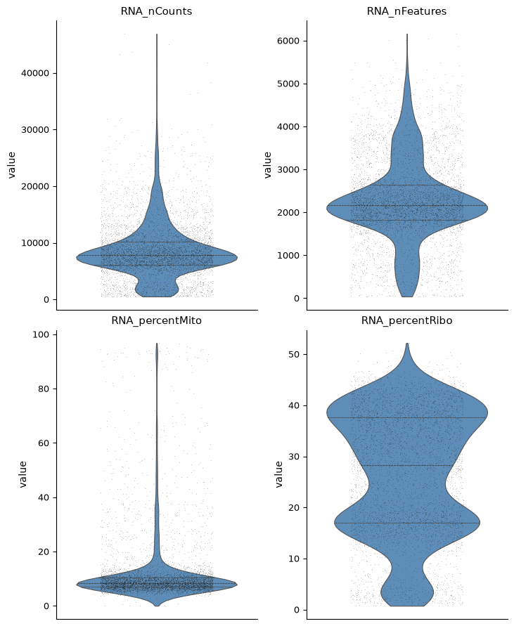
Started: 2026-10-11T18:55:06.009492Z | Wall time: 0.982 s
Each violin uses an immutable snapshot of I, so cells excluded when this store was opened are
not shown. Inspect low counts and few detected genes for low-complexity profiles, and high counts
for possible multiplets or high-RNA cell types. A distribution tail alone does not identify a
failed cell. Compare related metrics and the populations that a proposed cutoff would remove.
Start with automatic thresholds
qc.auto_filter uses the median absolute deviation (MAD), a measure of spread that is less
affected by extreme values than the standard deviation. Its default bounds are three scaled
MADs from the median. Counts and detected features use log1p values and two-sided bounds;
mitochondrial and ribosomal percentages use upper bounds only.
# Filter cells with the default robust thresholds.
automatic_selection = ds.qc.auto_filter(cell_selection=qc_cell_selection)

# Load the cells retained by automatic filtering.
automatic_mask = np.asarray(ds.artifacts.load(automatic_selection)["values"][:], dtype=bool)

# Count cells retained by automatic filtering.
print(f"Cells after automatic filtering: {int(automatic_mask.sum())}")

# Inspect the same quality measurements after automatic filtering.
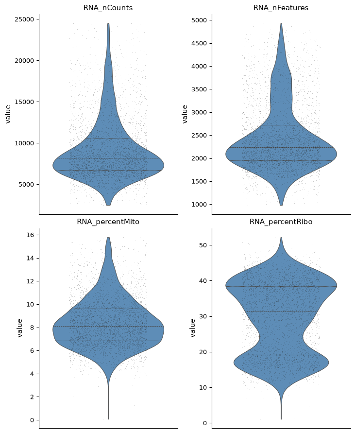
ds.plots.distribution(keys=qc_cols, cell_selection=automatic_selection)
Cells after automatic filtering: 4331
Started: 2026-10-11T18:55:06.995231Z | Wall time: 0.805 s
Compare these distributions with the input before accepting the result. Automatic bounds flag outliers from this population, not known damaged cells. Low-RNA and high-RNA populations may fall outside them even when their measurements are usable. Inspect which populations and samples would be lost, rather than accepting the filter because the distributions look narrower.
Choose manual thresholds when needed
Thresholds are dataset-specific.
The values below match the PBMC example in Identify PBMC populations with scRNA-seq.
Filtering returns a new immutable selection and leaves cell key I unchanged.
The named QC columns are read from current cell metadata when the method is called. If any
explicitly named column is absent, filtering raises an error instead of silently omitting it.
Mitochondrial and ribosomal patterns need matching feature names. If the store uses Ensembl IDs
instead of gene symbols, check those names before interpreting a missing or zero percentage.
# Count cells before applying manual thresholds.
n_before = int(ds.cells.fetch_all("I").sum())

# Define the manual count, feature, and mitochondrial thresholds.
manual_filter = {
    "attrs": ["RNA_nCounts", "RNA_nFeatures", "RNA_percentMito"],
    "highs": [15000, 4000, 15],
    "lows": [1000, 500, 0],
}

# Apply the manual thresholds to the input cells.
manual_selection = ds.qc.filter(**manual_filter)

# Load the cells retained by manual filtering.
manual_mask = np.asarray(ds.artifacts.load(manual_selection)["values"][:], dtype=bool)

# Report the input cell count.
print(f"Cells in input selection: {n_before}")

# Report the retained cell count.
print(f"Cells in filtered selection: {int(manual_mask.sum())}")

# Summarize the selected values and their spread.
pd.DataFrame({key: ds.cells.fetch_all(key)[manual_mask] for key in qc_cols}).describe()
Cells in input selection: 5025
Cells in filtered selection: 3948
| RNA_nCounts | RNA_nFeatures | RNA_percentMito | RNA_percentRibo | |
|---|---|---|---|---|
| count | 3948.000000 | 3948.000000 | 3948.000000 | 3948.000000 |
| mean | 8241.683384 | 2269.690983 | 8.422534 | 30.185056 |
| std | 2472.030006 | 542.209124 | 2.121822 | 10.211426 |
| min | 1057.000000 | 512.000000 | 0.076336 | 0.737101 |
| 25% | 6561.750000 | 1922.000000 | 6.892547 | 20.077556 |
| 50% | 7881.000000 | 2185.500000 | 8.195208 | 32.447885 |
| 75% | 9605.000000 | 2527.000000 | 9.721759 | 38.763019 |
| max | 14992.000000 | 3930.000000 | 14.975450 | 52.181596 |
Started: 2026-10-11T18:55:07.803099Z | Wall time: 0.141 s
The saved execution retains 3,948 of 5,025 input cells with these bounds, removing 1,077 (about 21%). This records the effect of the chosen thresholds; it is not a target removal rate for another dataset. Inspect the excluded cells as well as the retained summary before accepting that loss.
The automatic and manual selections are alternatives here. The doublet example below uses the
manual thresholds so it follows the same cells as the core PBMC workflow. To combine filters in
your own analysis, pass the previous result as cell_selection=.
Per-sample MAD filtering
Global bounds can penalize a sample whose count-depth distribution differs from the pooled distribution.
With sample_column, CyteArc calculates robust bounds within each sample using the median absolute deviation (MAD).
The PBMC teaching dataset has no biological sample column. Use a real sample column when the dataset contains multiple donors or batches. The call has the same immutable-selection contract as the global filter:
# Estimate quality thresholds separately for each sample.
sample_selection = ds.qc.auto_filter(
    cell_selection=qc_cell_selection,
    sample_column="sample_id",
)
This example needs a real sample_id column, which the PBMC dataset does not have.
Samples with fewer than 20 selected cells are retained with a warning because their bounds
cannot be estimated reliably. The same rule applies to a pooled selection with fewer than 20 cells.
The same options can be forwarded through the standard pipeline:
# Pass the sample-specific filtering choice through the pipeline.
ds.pipeline.run(
    filtering={"sample_column": "sample_id"},
)
RNA percentages and feature exclusions
Mitochondrial and ribosomal percentage columns measure the fraction of each cell’s counts matching configured gene-name patterns. The ribosomal pattern matches ribosomal protein genes, not the amount of ribosomal RNA. High mitochondrial percentages can accompany damaged cells, while both percentages can vary with cell type or state. Inspect them alongside counts and detected features before applying upper thresholds.
The default mitochondrial pattern is case-insensitive ^MT-.
It matches names such as MT-CO1 and mt-Co1 without including MTOR or metallothioneins.
Percentage columns are fixed when a store is first prepared. That first open for writing discards
any existing column with a percentage name, logs a warning, and computes the percentage from the
counts. Later opens keep the stored values when mito_pattern and ribo_pattern are omitted. An
explicit pattern that differs from the recorded one raises an error instead of replacing prepared
data. To apply a different pattern, import the data into a fresh store and pass the pattern on
its first open, or compute a separate quality_metric artifact as shown below.
For another gene set, create an explicit feature selection and calculate its percentage over an
explicit cell selection. The datastore method returns a quality_metric artifact and does not add
a cell column:
# Read the RNA feature names.
feature_names = ds.RNA.feats.fetch_all("names").astype(str)

# Select genes whose names start with HSP.
stress_features = ds.features.snapshot(
    from_assay="RNA",
    mask=np.char.startswith(feature_names, "HSP"),
)

# Calculate the selected genes' count percentage in each retained cell.
stress_percentage = ds.qc.feature_percentage(manual_selection, stress_features)

# Load the calculated percentages.
stress_values = np.asarray(ds.artifacts.load(stress_percentage)["values"][:])

# Summarize the selected values and their spread.
pd.Series(stress_values, name="percent stress features").describe()
count 3948.000000
mean 0.328236
std 0.130572
min 0.000000
25% 0.238440
50% 0.309681
75% 0.395623
max 1.531394
Name: percent stress features, dtype: float64Started: 2026-10-11T18:55:07.947670Z | Wall time: 0.724 s
Gene families excluded from the graph are a separate feature-selection decision. See Feature selection: choosing informative features for the default HVG blacklist and supported overrides.
Doublet scores
When two cells enter the same droplet, their transcripts can be assigned to one barcode. Such a doublet can combine markers from different lineages and resemble a new cell state. Doublets from similar cells are harder to distinguish from singlets by expression alone.
The pipeline builds a graph and clusters before calculating doublet scores. Most simulated doublets
pair cells from two different clusters (heterotypic_fraction, 0.8 by default), so scoring needs
a clustering with at least two clusters. The pipeline does not remove cells automatically. Here we
reuse the manual QC thresholds and the prepared PBMC example’s
500 genes, 15 PCs, and Leiden resolution 0.5. These are teaching-dataset settings, not the API
defaults. We skip cell-cycle scoring, Paris, and markers because they are not needed for this check.
# Run the graph and clustering steps needed for doublet scoring.
doublet_run = ds.pipeline.run(
    filtering={"method": "manual", **manual_filter},
    hvg_count=500,
    pca_dims=15,
    leiden={"partitions": [0.5]},
    cell_cycle=False,
    paris=False,
    doublets=True,
    markers=False,
)

# Keep the doublet-score artifact for further filtering.
doublets = doublet_run["doublets"]

# Read the doublet scores in the analysis cell order.
scores = np.asarray(doublet_run.cells.fetch("doublet_score"))

# Name the scores for summaries and plots.
scores_series = pd.Series(scores, name="doublet_score")

# Summarize the selected values and their spread.
scores_series.describe()
count 3948.000000
mean 0.103634
std 0.118792
min 0.000000
25% 0.019126
50% 0.060054
75% 0.152437
max 1.000000
Name: doublet_score, dtype: float64Started: 2026-10-11T18:55:08.674042Z | Wall time: 91.077 s
Locate high doublet scores on the embedding:
# Locate cells with high doublet scores on the UMAP.
ds.plots.embedding(run=doublet_run, color_by="doublet_score", sort_values=True)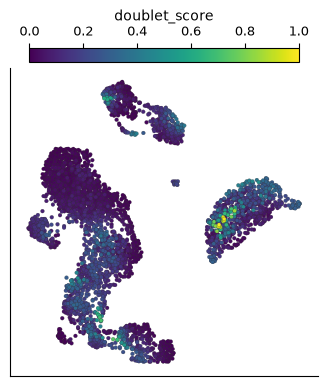
Started: 2026-10-11T18:56:39.753056Z | Wall time: 0.429 s
Higher doublet scores mark cells that map near simulated doublets. Inspect the score distribution before applying a cutoff:
# Plot the doublet-score distribution.
scores_series.plot(kind="hist", bins=40, xlabel="Doublet score")

# Display the completed figure.
plt.show()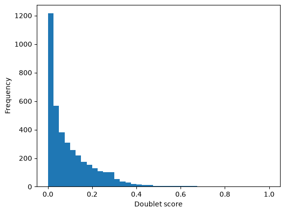
Started: 2026-10-11T18:56:40.184823Z | Wall time: 0.171 s
The score distribution and embedding should be reviewed together.
A threshold is study-dependent, and qc.doublets does not remove cells.
After choosing an upper bound from the score distribution, apply it as an additional filter.
The teaching cutoff below marks the upper 5% of scores on this PBMC run. A percentile always
selects an upper tail, even if there is no separate doublet population; it neither estimates a
doublet rate nor makes these scores probabilities. Choose a study-specific cutoff using the
score distribution, expected multiplet rate, and marker or sample evidence.
# Use the 95th percentile as this example's upper cutoff.
doublet_threshold = float(scores_series.quantile(0.95))

# Report the selected doublet-score cutoff.
print(f"Doublet threshold (95th percentile): {doublet_threshold:.4f}")

# Count cells excluded by the cutoff.
print(f"Cells above threshold: {int((scores > doublet_threshold).sum())}")
Doublet threshold (95th percentile): 0.3148
Cells above threshold: 198
Started: 2026-10-11T18:56:40.358523Z | Wall time: 0.007 s
Compose the upper bound with the score artifact’s stored input selection. This retains scores at the bound and leaves live metadata unchanged:
# Retain cells whose score is at or below the chosen cutoff.
doublet_filtered = ds.select_cells(doublets, high=doublet_threshold, keep_bounds=True)

# Count the cells retained after applying the cutoff.
int(np.asarray(ds.artifacts.load(doublet_filtered)["values"][:]).sum())3750Started: 2026-10-11T18:56:40.368588Z | Wall time: 0.053 s
select_cells reads the canonical array of a cell-aligned artifact kind, here values of the
doublet_score, and refuses kinds that the table of cell-aligned kinds does not list
(Cell-aligned result kinds). low and high define the retained range of numeric values. By
default it composes with the source artifact’s selection; cell_selection= can narrow that input
further but cannot add cells absent from the source.
ATAC quality control
CyteArc initializes per-cell ATAC fragment or cut-site counts and accessible-peak counts, and it records per-peak detection statistics for explicit prevalent-peak selection.
features.prevalent_peaks returns the peak selection used for LSI and graph construction.
CyteArc does not currently calculate FRiP or TSS enrichment, so those metrics must be imported as metadata or computed with an external tool rather than implied by the available columns.
ADT and multimodal quality control
ADT panels often include control antibodies that should be excluded with an explicit feature selection after their names are inspected. RNA, ADT, and HTO assays share one cell table, so one cell-selection artifact can be passed to each compatible assay operation. Check whether an RNA-driven filter is appropriate for the protein question before reusing it automatically. Hashtag demultiplexing is covered separately in HTO demultiplexing.
Common mistakes and limitations
Treating thresholds as portable: values are specific to a dataset’s distributions, and pooling samples with different count depths under one global bound can penalize the shallower samples. Inspect distributions first, and use
sample_columnwhen samples differ.Treating doublet scoring as automatic cleanup:
qc.doubletsonly scores, so removal needs an explicit selection built from those scores; scoring itself requires the graph and clustering to exist first, and the teaching 95th-percentile cutoff is an illustrative upper tail, not a true doublet rate.Reading ATAC quality beyond what CyteArc currently provides: stores carry fragment or cut-site counts and accessible-peak counts, not FRiP or TSS enrichment; import those metrics as metadata or compute them externally.