Quick start - CyteArc

Start by plotting a prepared analysis of 100,000 cells from Tabula Sapiens. You do not need your own count file. Then use the same workflow to analyze your own RNA data.

Complete the installation with the extra dependencies first.

Try a prepared example¶

Download an already analyzed sample from Tabula Sapiens. The first download is about 1.56 GB. It retains all 24 donors, with sampling proportional to each tissue and donor’s contribution. For a smaller download, start with the PBMC walkthrough. To explore the full 1.1-million-cell atlas without downloading the full count matrix, use Explore a remote dataset.

# Import CyteArc for the prepared atlas example.
import cytearc

# Keep download progress and routine logs out of the saved output.
cytearc.configure_output(level="WARNING", progress=False)

# Download the prepared example, including its saved analysis.
dataset = cytearc.cytebase.connect("cytearc_docs").download_dataset(
    "tabula_sapiens_100k", destination="cytearc_datasets", zarr=True
)

Started: 2026-10-11T18:54:39.870059Z | Wall time: 21.179 s

Open the downloaded store and inspect its saved analysis.

# Open the datastore for the following analysis.
ds = cytearc.DataStore(f"{dataset}/data.zarr", min_features_per_cell=-1)

# Open the saved analysis and retain its exact results.
run = ds.pipeline.open(label="docs_default")

# Inspect the store's assays and dimensions.
ds

DataStore has 100000 (100000) cells with 1 assays: RNA
   Cell metadata:
            'I', 'ids', 'names', '10X_run', 'RNA_nCounts', 
            'RNA_nFeatures', 'RNA_percentMito', 'RNA_percentRibo', '_scvi_batch', '_scvi_labels', 
            'ambient_removal', 'anatomical_position', 'assay', 'assay_ontology_term_id', 'broad_cell_class', 
            'cdna_plate', 'cdna_well', 'cell_type', 'cell_type_ontology_term_id', 'compartment', 
            'development_stage', 'development_stage_ontology_term_id', 'disease', 'disease_ontology_term_id', 'donor_assay', 
            'donor_id', 'donor_method', 'donor_tissue', 'donor_tissue_assay', 'ethnicity_original', 
            'free_annotation', 'is_primary_data', 'library_plate', 'manually_annotated', 'method', 
            'n_genes_by_counts', 'notes', 'observation_joinid', 'pct_counts_ercc', 'pct_counts_mt', 
            'published_2022', 'replicate', 'sample_id', 'sample_number', 'scvi_leiden_donorassay_full', 
            'self_reported_ethnicity', 'self_reported_ethnicity_ontology_term_id', 'sex', 'sex_ontology_term_id', 'suspension_type', 
            'tissue', 'tissue_in_publication', 'tissue_ontology_term_id', 'tissue_type', 'total_counts', 
            'total_counts_ercc', 'total_counts_mt'
   RNA assay has 60606 features and following metadata:
            'I', 'ids', 'names', '_index', 'dropOuts', 
            'ercc', 'feature_biotype', 'feature_length', 'feature_reference', 'feature_type', 
            'genome', 'mean', 'mean_counts', 'mt', 'nCells', 
            'n_cells_by_counts', 'pct_dropout_by_counts', 'std', 'total_counts'

Started: 2026-10-11T18:55:01.054082Z | Wall time: 6.323 s

pipeline.open reads saved results; pipeline.run computes an analysis. Here docs_default is the name of the prepared example. It used 2,000 variable genes, 30 PCs, and 21 neighbours, so its labels and plots need not match a new run with the current defaults.

# Color the prepared atlas embedding by its saved clusters.
ds.plots.embedding(run=run, color_by="clusters", show_legend=False, point_size=0.5)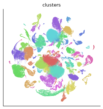

UMAP of 100,000 Tabula Sapiens cells colored by saved RNA clusters. Each color marks a cluster, not an assigned cell type.

Started: 2026-10-11T18:55:07.381263Z | Wall time: 2.375 s

Each colour marks a cluster of cells with similar RNA profiles. A cluster number is not a cell type. The source’s cell-type annotations remain in ds.cells; the clusters shown here come from the CyteArc analysis. Continue with the smaller PBMC walkthrough to work through each step and compare marker genes. For another input format, see Import and export; for a familiar workflow translation, see CyteArc for Scanpy users or CyteArc for Seurat users.

Analyze your own RNA-seq data¶

For a filtered Cell Ranger H5 file, convert the counts to a CyteArc store and run the pipeline:

# Import CyteArc to open and analyze your count store.
import cytearc

# Read the count matrix and its cell and feature identifiers.
reader = cytearc.CrH5Reader("filtered_feature_bc_matrix.h5")

# Write the prepared counts and metadata to the new store.
cytearc.CrToZarr(reader, zarr_loc="analysis.zarr").dump()

# Open the datastore for the following analysis.
ds = cytearc.DataStore("analysis.zarr")

# Run the default RNA analysis and retain its results.
run = ds.pipeline.run(label="baseline")

# Color the new RNA embedding by its selected clusters.
ds.plots.embedding(run=run, color_by="clusters")

Use a new or empty output path for conversion. A writer raises FileExistsError for a path that already holds data. Pass overwrite=True to replace an earlier conversion that no DataStore has opened; once opened, a store is prepared and is never replaced, so delete it yourself or choose another path. The pipeline uses CyteArc’s default settings for filtering, feature selection, PCA, neighbours, UMAP, clustering, and marker search. It also scores cell cycle and doublets. These settings are a starting point; review Quality control across assays and the marker evidence before interpreting a new dataset.

run holds the results of this analysis. Keep it to make plots and read marker tables without repeating the computation. Each named run needs a new label; reopen a completed one with ds.pipeline.open(label="baseline").

For control over individual steps, use ds.features, ds.reduction, ds.graph, ds.embeddings, ds.clusters, and ds.markers. The graph tutorial follows this route with explicit inputs and saved results. These methods use the same computations as the pipeline.