Single-cell readouts on single genes can be sparse and heavily noisy. This is often driven by dropout, which can zero out a marker in cells that express it, and then one highly expressed gene can dominate expression. Gene-set scoring fixes this by collapsing a whole program; a pathway, a cell state, a lineage signature; into one number per cell that is more robust than any member gene alone.
CyteArc offers two ways to compute that number. WAGGR (Weighted Aggregate) takes a weighted mean of normalized gene expression, so strongly expressed genes can pull harder and can push in opposite directions. AUCell ignores expression values entirely after ranking each cell’s genes, then measures how early the signature’s targets appear among the top ranks, with its scores ranging from 0 to 1. WAGGR can be used to gain an idea of the magnitude of a program, whereas AUCell can tell you about rank recovery. Rank recovery can be conceptualized as how early the signature of interest appears among that cell’s top-ranked genes.
Load the prepared dataset
We first begin by loading in the prepared dataset. For context, when we do our activity scoring, the data is streamed directly from the raw counts: AUCell ranks those raw counts, while WAGGR applies library-size normalization for its own scoring function.
# Import tools for writing a temporary GMT file.
from pathlib import Path
from tempfile import TemporaryDirectory

# Import plotting and table tools for inspecting the scores.
import matplotlib.pyplot as plt
import pandas as pd

# Import CyteArc's datastore and gene-set scoring methods.
import cytearc

# Keep warnings visible while hiding routine progress messages.
cytearc.configure_output(level='WARNING', progress=False)

# Download the prepared PBMC store and its saved analysis.
dataset = cytearc.cytebase.connect("cytearc_docs").download_dataset(
    'tenx_5K_pbmc_rnaseq',
    destination='cytearc_datasets',
    zarr=True,
)

# Open the store so scoring can save its results.
ds = cytearc.DataStore(f'{dataset}/data.zarr', nthreads=4)

# Reuse the saved analysis and its selected cells.
run = ds.pipeline.open(label='docs_default')

# Inspect the opened assays and their dimensions.
ds
DataStore has 3948 (5025) cells with 1 assays: RNA
Cell metadata:
'I', 'ids', 'names', 'RNA_G2M_score', 'RNA_S_score',
'RNA_UMAP1', 'RNA_UMAP2', 'RNA_cell_cycle_phase', 'RNA_clusters', 'RNA_doublet_score',
'RNA_leiden_cluster', 'RNA_nCounts', 'RNA_nFeatures', 'RNA_paris_cluster', 'RNA_percentMito',
'RNA_percentRibo'
RNA assay has 33538 features and following metadata:
'I', 'ids', 'names', 'dropOuts', 'feature_type',
'genome', 'nCells'Started: 2026-10-11T18:54:48.982669Z | Wall time: 11.992 s
Read and inspect gene sets
For your own analysis, replace these demonstration signatures with your own Gene Matrix Transposed (GMT) file. The file stores one gene program per line.
# Keep the demonstration GMT file in a temporary folder.
input_directory = TemporaryDirectory()

# Choose the filename for the three PBMC signatures.
gmt_path = Path(input_directory.name) / 'pbmc_signatures.gmt'

# Write five target genes for each demonstration signature.
gmt_path.write_text(
    'T_cell\tna\tCD3D\tCD3E\tTRAC\tLTB\tIL7R\n'
    'B_cell\tna\tMS4A1\tCD79A\tCD37\tCD74\tHLA-DRA\n'
    'Myeloid\tna\tLST1\tS100A8\tS100A9\tCTSS\tFCER1G\n',
    encoding='utf-8',
)

# Read the GMT as a table of signature names and target genes.
gene_sets = cytearc.read_gmt(gmt_path)

# Inspect the genes assigned to each signature.
gene_sets| source | target | |
|---|---|---|
| 0 | T_cell | CD3D |
| 1 | T_cell | CD3E |
| 2 | T_cell | TRAC |
| 3 | T_cell | LTB |
| 4 | T_cell | IL7R |
| 5 | B_cell | MS4A1 |
| 6 | B_cell | CD79A |
| 7 | B_cell | CD37 |
| 8 | B_cell | CD74 |
| 9 | B_cell | HLA-DRA |
| 10 | Myeloid | LST1 |
| 11 | Myeloid | S100A8 |
| 12 | Myeloid | S100A9 |
| 13 | Myeloid | CTSS |
| 14 | Myeloid | FCER1G |
Started: 2026-10-11T18:55:00.979846Z | Wall time: 0.027 s
Targets are matched to active RNA feature names without case sensitivity, meaning that any match regardless of capitalization will be selected. Missing targets do not need to be removed from the input table, as CyteArc automatically handles this. A target that matches several active features, such as a gene symbol shared by two feature IDs, is ambiguous and is ignored with a warning by default.
# Normalize gene-name case before checking signature overlap.
available = {str(name).upper() for name in ds.RNA.feats.fetch_all('names')}

# Mark each target whose name occurs in this assay.
matched_targets = gene_sets.assign(matched=gene_sets['target'].str.upper().isin(available))

# Compare matched and total target counts for each signature.
matched_targets.groupby('source')['matched'].agg(['sum', 'count'])| sum | count | |
|---|---|---|
| source | ||
| B_cell | 5 | 5 |
| Myeloid | 5 | 5 |
| T_cell | 5 | 5 |
Started: 2026-10-11T18:55:01.009559Z | Wall time: 0.057 s
In our case, all five genes in each of the three signatures are present in the dataset.
Start with WAGGR
WAGGR calculates a weighted mean of library-size-normalized expression by default.
When the input has no weight column, every target gene has weight one.
tmin is the minimum number of matched genes a signature needs to be scored; anything below it is skipped. Our sample gene sets have only five genes each, so tmin=3 lets a signature survive one or two missing genes, where the default of five would drop it outright.
This comparison uses the complete assay feature universe for both methods:
# Reuse the cells selected by the saved analysis.
cell_selection = run['analysis_cell_selection']

# Include every RNA feature in the scoring universe.
all_features = ds.features.universe(from_assay='RNA')

# Show the number of cells and genes used by both methods.
{'cells': int(run.cells.fetch_all('I').sum()), 'genes': ds.RNA.feats.N}
{'cells': 3948, 'genes': 33538}Started: 2026-10-11T18:55:01.069024Z | Wall time: 0.182 s
# Aggregate normalized expression for each demonstration signature.
waggr = ds.scores.waggr(
    gene_sets,
    cell_selection,
    features=all_features,
    tmin=3,
)

# Keep the same signature order throughout the comparison.
score_sources = ['T_cell', 'B_cell', 'Myeloid']

# Load only the three signatures compared in this tutorial.
waggr_result = ds.scores.load(waggr, sources=score_sources)

# Materialize the three score columns as a table.
waggr_scores = pd.DataFrame(
    waggr_result.data.compute(),
    columns=list(waggr_result.source_names),
)

# Inspect the range and median of each signature's WAGGR scores.
waggr_scores.describe().loc[['min', '50%', 'max']]| T_cell | B_cell | Myeloid | |
|---|---|---|---|
| min | 0.000000 | 0.000000 | 0.000000 |
| 50% | 0.562968 | 0.172488 | 0.047424 |
| max | 2.551281 | 7.278358 | 25.161978 |
Started: 2026-10-11T18:55:01.253949Z | Wall time: 1.029 s
The results from WAGGR are not confined from 0 to 1 like AUCell.
Score rank recovery with AUCell
Since AUCell scores each cell by recovery among its top-ranked genes, it first needs to know what universe to rank. The required features argument sets that universe: here all_features ranks the complete gene list, but AUCell only uses the top 5% of genes to calculate its recovery.
# Score recovery of each signature among the top-ranked genes.
aucell = ds.scores.aucell(
    gene_sets,
    cell_selection,
    features=all_features,
    tmin=3,
)

# Load AUCell scores in the same signature order as WAGGR.
aucell_result = ds.scores.load(aucell, sources=score_sources)

# Materialize the three AUCell score columns as a table.
aucell_scores = pd.DataFrame(
    aucell_result.data.compute(),
    columns=list(aucell_result.source_names),
)

# Inspect the range and median of each signature's AUCell scores.
aucell_scores.describe().loc[['min', '50%', 'max']]| T_cell | B_cell | Myeloid | |
|---|---|---|---|
| min | 0.000000 | 0.000000 | 0.000000 |
| 50% | 0.678495 | 0.308961 | 0.075030 |
| max | 0.933692 | 0.975508 | 0.985544 |
Started: 2026-10-11T18:55:02.286492Z | Wall time: 15.174 s
An AUCell score of 0 means no signature genes are recovered before the top-rank cutoff; a gene exactly at the cutoff contributes no area. A score of 1 means the signature achieves the maximum possible recovery at the top of that cell’s ranking.
Visualize AUCell and WAGGR
To visualize the results from AUCell, we can simply plot the recovery score on a UMAP of the cells.
# Read the saved UMAP coordinates in the score table's cell order.
umap = run.cells.to_pandas_dataframe(['umap_1', 'umap_2'])

# Create one panel per signature.
figure, axes = plt.subplots(1, 3, figsize=(12, 4))

# Map each signature's AUCell score onto the same UMAP.
for axis, source in zip(axes, score_sources, strict=True):

    # Use the common zero-to-one scale for every signature.
    points = axis.scatter(
        umap['umap_1'],
        umap['umap_2'],
        c=aucell_scores[source],
        s=3,
        vmin=0,
        vmax=1,
    )

    # Identify the signature shown in the panel.
    axis.set_title(f'{source} AUCell')

    # Label the score scale used to color the cells.
    figure.colorbar(points, ax=axis, label='AUCell score')

# Make room for panel titles and color scales.
figure.tight_layout()

# Display the three signature maps.
plt.show()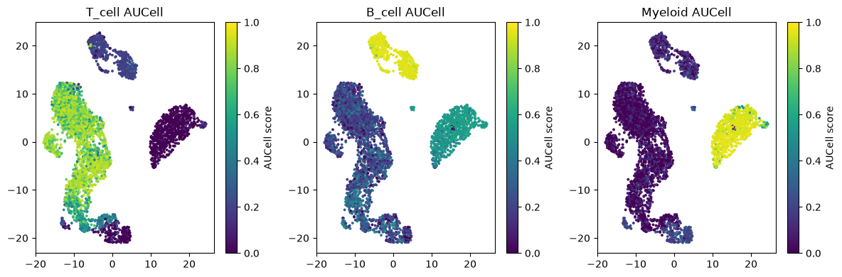
Started: 2026-10-11T18:55:17.466387Z | Wall time: 0.706 s
AUCell scores highlight lineage-consistent regions: T cell, B cell, and Myeloid scores peak in separate parts of the UMAP when those populations are present.
To compare both methods, take the Myeloid signature for example: we can create a table comparing the results; remember, their numerical scales differ.
# Align the Myeloid signature's scores from both methods by cell.
myeloid_compare = pd.DataFrame(
    {
        'Myeloid_WAGGR': waggr_scores['Myeloid'],
        'Myeloid_AUCell': aucell_scores['Myeloid'],
    }
)

# Compare the distributions without assuming a shared numerical scale.
myeloid_compare.describe()| Myeloid_WAGGR | Myeloid_AUCell | |
|---|---|---|
| count | 3948.000000 | 3948.000000 |
| mean | 1.246021 | 0.229799 |
| std | 3.026997 | 0.343544 |
| min | 0.000000 | 0.000000 |
| 25% | 0.022398 | 0.000000 |
| 50% | 0.047424 | 0.075030 |
| 75% | 0.137805 | 0.187366 |
| max | 25.161978 | 0.985544 |
Started: 2026-10-11T18:55:18.176162Z | Wall time: 0.019 s
We can also compare WAGGR and AUCell scores for the Myeloid signature across all selected cells in a scatter plot.
# Create an axis for the comparison between scoring methods.
figure, axis = plt.subplots(figsize=(4, 4))

# Plot one point per cell using its two Myeloid signature scores.
axis.scatter(
    myeloid_compare['Myeloid_WAGGR'],
    myeloid_compare['Myeloid_AUCell'],
    s=4,
    alpha=0.35,
)

# Label the expression-based score on the horizontal axis.
axis.set_xlabel('Myeloid WAGGR')

# Label the rank-recovery score on the vertical axis.
axis.set_ylabel('Myeloid AUCell')

# Display the comparison between the two scoring methods.
plt.show()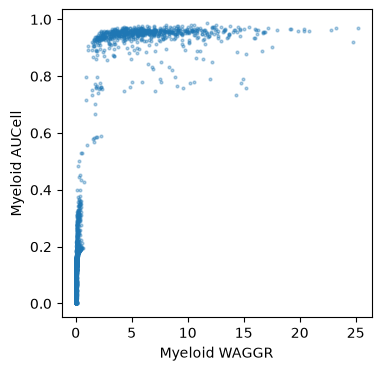
Started: 2026-10-11T18:55:18.197077Z | Wall time: 0.121 s
Look for cells with high scores under both methods and cells where the methods disagree.
Optional: Use a signature with weights
Add weights when the WAGGR source gives some genes more say than others: amplifying strong genes, silencing weak ones, or setting genes against each other in opposite directions. To adjust for this, add a weight column to the input table, as without one, every gene counts equally at weight one. WAGGR’s default mode="wmean" divides the weighted sum by the sum of absolute weights, keeping scores comparable across signatures of different sizes, while mode="wsum" leaves the total unscaled, so comparability falls.
Common mistakes and limitations
Restricting AUCell’s ranking universe: recovery is measured within the top 5% of whatever list
featuresprovides, so scoring against a subset such as highly variable genes shifts background ranks and inflates or skews the score. Rank against the full feature universe.Letting
tminprune a signature silently: unmatched or ambiguous targets drop out, and a signature left with fewer thantminmatched targets is skipped entirely rather than scored on its surviving subset; if no signatures remain, scoring raises an error.Comparing WAGGR scores across transformations: WAGGR values are unbounded and sensitive to
log_transform,wmeanvs.wsum, and library normalization, so comparing runs with different settings, or WAGGR directly against AUCell’s bounded 0-to-1 scores, confounds scaling with biology.