CyteBase case study: COVID-19 blood

This page follows one research question from start to finish, using a published dataset from CyteBase:

How does the peripheral blood of COVID-19 patients differ from that of healthy donors?

It finds a disease-versus-control dataset in the catalog, opens it remotely, and answers the question with cell metadata and about two dozen genes. The H5AD is never downloaded: CyteArc reads metadata and the needed count blocks over the network. Explore CyteBase introduces the catalog and the SDK calls used here.

The saved results on this page were built with the CyteBase October 2026 release (2610), published in the public Nygen/cytebase-2610 bucket, which readers can access without credentials.

Use the page download menu to save the source notebook.

Install CyteArc’s SDK and required dependencies in your notebook environment:

# Install the CyteBase connector and a notebook environment.
uv pip install --prerelease allow 'cytearc[cytebase]' jupyterlab

Explore CyteBase describes bucket selection and credentials for private buckets.

Dataset¶

The dataset is Wilk et al. (2020), Nature Medicine, Wilk et al. (2020): Seq-Well profiling of peripheral blood mononuclear cells (PBMCs) from patients hospitalized with COVID-19 and from healthy donors. It was curated and distributed by CZ CELLxGENE Discover (CZI Cell Science Program et al., Nucleic Acids Research 2025, Abdulla et al. (2024)). Cite both the original study and CELLxGENE Discover when you use these data. All cell-type labels below are the published annotations; this page does not re-cluster or re-annotate.

The setup cell switches off CyteArc’s progress bars and logs only warnings, to keep the output readable. It also silences huggingface_hub retry messages, which can include full request URLs.

# Import tools for catalog access, donor summaries, and statistical comparisons.
import logging

import numpy as np
import pandas as pd
from IPython.display import Markdown, display
from scipy.stats import mannwhitneyu, spearmanr

import cytearc
from cytearc import cytebase
from cytearc.plotting import CategoricalScale, CellField, NormalizationSpec

# Keep routine progress messages out of the teaching output.
cytearc.configure_output(level="WARNING", progress=False)

# HF retry messages include request URLs; keep them out of shared outputs.
logging.getLogger("huggingface_hub").setLevel(logging.ERROR)

# Keep printed tables wide enough for the selected metadata.
pd.set_option("display.width", 160)

# Connect to the October 2026 release used for this page's saved results.
catalog = cytebase.Catalog(version="2610")

Started: 2026-10-12T13:56:00.408554Z | Wall time: 3.753 s

Find the dataset and open it remotely¶

Catalog() keeps a small, checksum-verified DuckDB copy of the catalog on your machine; searching it does not touch any count data. Search by author and topic rather than typing an ID by hand.

# Search the catalog for the dataset used in this example.
matches = catalog.search("wilk sars cov 2", ready_only=True, max_cell_chars=None)

# Summarize matching cohorts without letting full IDs dominate the table.
match_preview = matches.to_markdown(
    columns=["cytebase_id", "title", "cell_count"], max_cell_chars=32
)

# Display the cohort preview; result rows retain their complete identifiers.
display(Markdown(match_preview))

# Stop if the published COVID-19 cohort is unavailable.
if not matches:
    raise RuntimeError("The Wilk COVID-19 dataset is not ready in this catalog")

# Keep the dataset identifier returned by the catalog.
dataset_id = matches[0]["cytebase_id"]

# Read the dataset's scientific metadata and citation.
entry = catalog.dataset(dataset_id)

# Inspect the dataset record and source citation.
entry

Started: 2026-10-12T13:56:04.163839Z | Wall time: 6.605 s

entry is a catalog record: title, citation, CELLxGENE links, size, and ontology labels. Displaying it reads the catalog and the dataset’s build record, not the Zarr store.

open_datastore validates the published build and returns a read-only DataStore. Only small metadata files are fetched now; counts stay in the bucket until a gene is requested. The CELLxGENE UMAP was imported with the data, so it can be plotted directly instead of recomputing an embedding.

# Open the datastore for the following analysis.
ds = catalog.open_datastore(entry.id)

# Inspect the remote datastore dimensions and assays.
print(ds)

# List the imported embeddings before selecting the UMAP.
print("\nImported embeddings:", sorted(cytebase.embeddings(ds)))

# Select the imported UMAP without recomputing its coordinates.
umap_ref = cytebase.embedding(ds, "X_umap")

DataStore has 44721 (44721) cells with 1 assays: RNA
   Cell metadata:
            'I', 'ids', 'names', 'Admission', 'DPS', 
            'DTF', 'HLA1', 'IFN1', 'RNA_nCounts', 'RNA_nFeatures', 
            'RNA_percentMito', 'RNA_percentRibo', 'Ventilated', 'assay', 'assay_ontology_term_id', 
            'cell.type.coarse', 'cell.type.fine', 'cell_type', 'cell_type_ontology_term_id', 'development_stage', 
            'development_stage_ontology_term_id', 'disease', 'disease_ontology_term_id', 'donor_id', 'is_primary_data', 
            'nCount_RNA', 'nCount_SCT', 'nFeature_RNA', 'nFeature_SCT', 'observation_joinid', 
            'percent.mt', 'percent.rpl', 'percent.rps', 'percent.rrna', 'self_reported_ethnicity', 
            'self_reported_ethnicity_ontology_term_id', 'seurat_clusters', 'sex', 'sex_ontology_term_id', 'singler', 
            'suspension_type', 'tissue', 'tissue_ontology_term_id', 'tissue_type'
   RNA assay has 24505 features and following metadata:
            'I', 'ids', 'names', 'dropOuts', 'feature_biotype', 
            'feature_length', 'feature_reference', 'feature_type', 'nCells'


Imported embeddings: ['X_umap']

Started: 2026-10-12T13:56:10.770728Z | Wall time: 26.819 s

Study design from metadata alone¶

Besides the standard CELLxGENE fields (cell_type, disease, donor_id, and so on), the store keeps the study’s own columns: Ventilated and Admission (clinical status), DPS (days post symptom onset, 0 for healthy donors), the authors’ coarse and fine labels (cell.type.coarse, cell.type.fine), and per-cell scores such as IFN1.

Read only the columns needed into pandas. This reads cell metadata, not the expression matrix. Then summarize one row per donor.

# Choose the study-design and annotation fields needed below.
columns = [
    "cell_type",
    "cell.type.coarse",
    "disease",
    "donor_id",
    "Ventilated",
    "Admission",
    "DPS",
    "sex",
    "development_stage",
    "IFN1",
]

# Read cell metadata and index it by cell ID.
meta = ds.cells.to_pandas_dataframe(["ids", *columns], key="I").set_index("ids")

# Check how many cells and metadata columns were loaded.
print(f"{len(meta):,} cells, {meta.shape[1]} metadata columns read")

44,721 cells, 10 metadata columns read

Started: 2026-10-12T13:56:37.591507Z | Wall time: 13.035 s

Summarize clinical metadata once per donor.

# Combine distinct donor metadata values without hiding repeated samples.
def distinct(values):
    return " / ".join(map(str, sorted(values.unique())))


# Summarize the study metadata and cell count per donor.
donors = meta.groupby("donor_id").agg(
    disease=("disease", "first"),
    ventilated=("Ventilated", distinct),
    admission=("Admission", distinct),
    days_post_symptoms=("DPS", distinct),
    sex=("sex", "first"),
    age=("development_stage", "first"),
    cells=("disease", "size"),
)

# Inspect one clinical and cell-count summary per donor.
donors

	disease	ventilated	admission	days_post_symptoms	sex	age	cells
donor_id
C1	COVID-19	NonVent / Vent	ICU	9 / 11	male	seventh decade stage	8362
C2	COVID-19	NonVent	ICU	16	male	fifth decade stage	1735
C3	COVID-19	Vent	ICU	9	male	fourth decade stage	6545
C4	COVID-19	Vent	ICU	9	male	fourth decade stage	3688
C5	COVID-19	NonVent	ICU	15	male	sixth decade stage	2507
C6	COVID-19	Vent	ICU	2	male	80 year-old and over stage	1893
C7	COVID-19	NonVent	Floor	12	male	third decade stage	3364
H1	normal	Healthy	N/A	0	female	49-year-old stage	2100
H2	normal	Healthy	N/A	0	male	49-year-old stage	1941
H3	normal	Healthy	N/A	0	female	36-year-old stage	2306
H4	normal	Healthy	N/A	0	male	49-year-old stage	5136
H5	normal	Healthy	N/A	0	male	48-year-old stage	3146
H6	normal	Healthy	N/A	0	male	37-year-old stage	1998

Started: 2026-10-12T13:56:50.628400Z | Wall time: 0.032 s

The design is small: 7 COVID-19 patients (C1 to C7) and 6 healthy donors (H1 to H6), mostly male. Six patients were in intensive care and one (C7) on a general ward. C1 contributes two samples: day 9 (not ventilated) and day 11 (ventilated). The donor, not the cell, is the biological replicate, which matters for every comparison below.

Cell counts per donor range from about 1,700 to 8,400. The CELLxGENE cell_type column uses Cell Ontology names; the authors’ cell.type.coarse column groups them into 13 shorter labels, which the compact figures use. Each ontology label maps to exactly one coarse label:

# Count cells of each published type in each condition.
by_type = pd.crosstab(meta["cell_type"], meta["disease"])

# Match each detailed cell type to the authors' coarse label.
coarse_labels = meta.groupby("cell_type")["cell.type.coarse"].first()

# Place each coarse label beside its detailed cell-type counts.
by_type.insert(0, "coarse label", coarse_labels)

# Compare condition counts with the authors' shorter cell-type labels.
by_type.sort_values(["coarse label", "COVID-19"], ascending=[True, False])

disease	coarse label	COVID-19	normal
cell_type
B cell	B	1715	1966
class switched memory B cell	B	1313	28
CD14-positive monocyte	CD14 Monocyte	8285	2054
monocyte	CD16 Monocyte	433	915
CD4-positive, alpha-beta memory T cell	CD4 T	2890	1208
naive T cell	CD4 T	2224	1616
CD4-positive, alpha-beta T cell	CD4 T	448	11
CD8-positive, alpha-beta memory T cell	CD8 T	3312	2753
effector CD8-positive, alpha-beta T cell	CD8 T	565	132
conventional dendritic cell	DC	252	204
granulocyte	Granulocyte	420	110
neutrophil	Granulocyte	250	51
natural killer cell	NK	2150	4707
IgG plasmablast	PB	1087	20
IgA plasmablast	PB	890	66
platelet	Platelet	464	63
erythrocyte	RBC	1259	178
gamma-delta T cell	gd T	45	403
plasmacytoid dendritic cell	pDC	92	142

Started: 2026-10-12T13:56:50.661914Z | Wall time: 0.029 s

Raw cell counts already hint at differences (for example, many more plasmablasts from COVID-19 samples), but they mix biology with how many cells each donor contributed. The “Composition per donor” section returns to this with per-donor proportions.

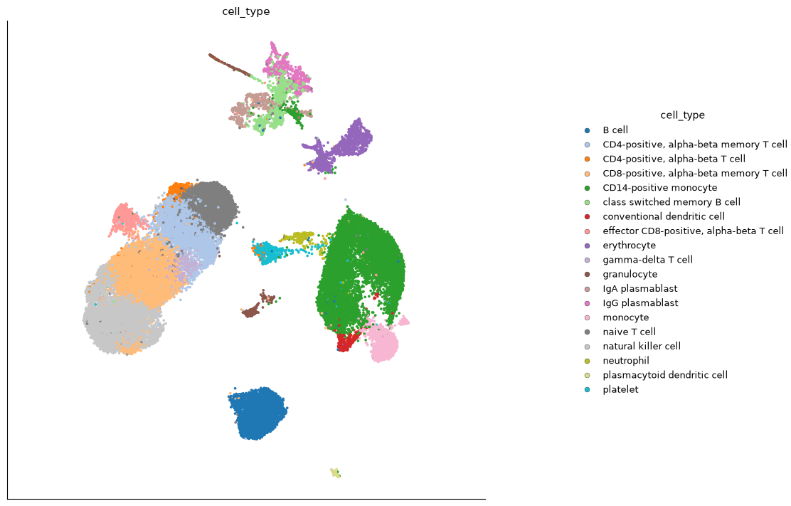
The published UMAP¶

ds.plots.embedding(layout=umap_ref, ...) draws the imported CELLxGENE coordinates. First, the full Cell Ontology annotation:

# Show the published Cell Ontology labels on the imported UMAP.
ds.plots.embedding(
    layout=umap_ref,
    color_by="cell_type",
    legend_loc="right",
    figsize=(12, 7),
)

Imported blood-cell UMAP colored by published Cell Ontology labels, including lymphocytes, monocytes, dendritic cells, plasmablasts, erythrocytes, and platelets.

Started: 2026-10-12T13:56:50.692116Z | Wall time: 13.504 s

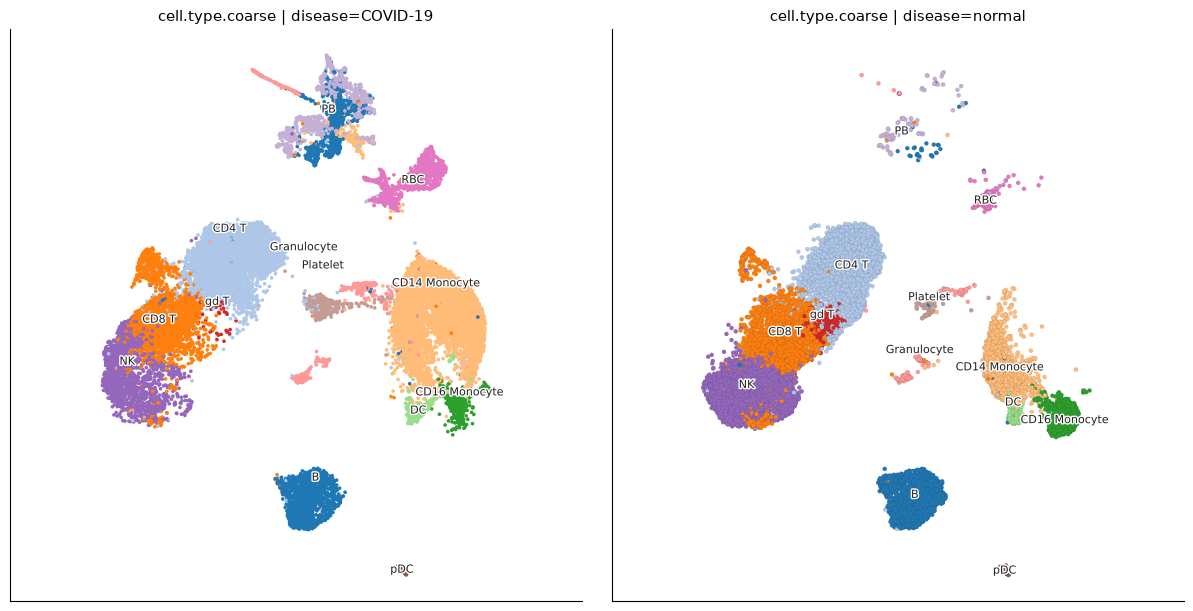
Splitting the same layout by condition with facet_by shows where each group’s cells fall. Labels are the authors’ coarse types.

# Compare the two conditions on matching UMAP panels.
ds.plots.embedding(
    layout=umap_ref,
    color_by="cell.type.coarse",
    facet_by="disease",
    figsize=(12, 6),
)

Matching UMAP panels split COVID-19 and healthy cells by condition. Plasmablasts are more abundant in the COVID-19 panel, and the two conditions occupy different parts of the CD14 monocyte region.

Started: 2026-10-12T13:57:04.197471Z | Wall time: 9.163 s

Two differences stand out. The plasmablast (PB) island at the top is well populated in COVID-19 but sparse in healthy blood. The CD14 monocyte island is shifted: healthy monocytes sit on its left side, while most COVID-19 monocytes occupy the right side. This suggests a condition-associated difference within the annotated cell type, but the layout alone does not establish its cause. The gene-expression comparisons below examine that difference.

These panels show where the cells lie, but donors contribute different numbers of cells. Next, compare proportions within each donor. For highlighting populations, see Core plotting features.

Composition per donor¶

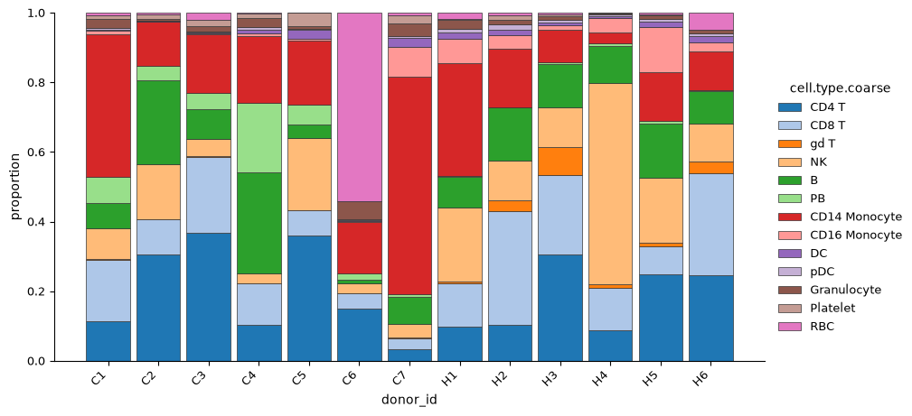
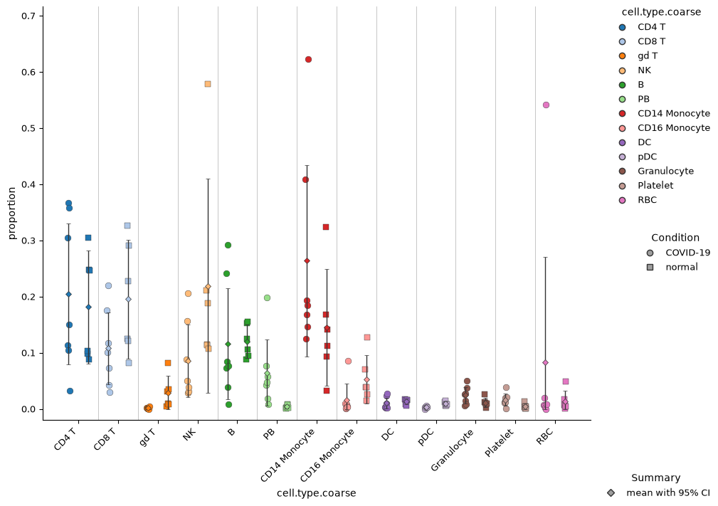
Proportions are computed within each donor, so a donor with many cells does not dominate. The stacked view shows the composition of the cells retained in this dataset for each donor, rather than absolute cell numbers in blood. With condition_by, the kind="per_sample" view then places one point per donor for each condition: circles for COVID-19 and squares for healthy donors, with the group mean and 95% confidence interval as a diamond.

# Use the same cell-type order across composition figures.
coarse_order = [
    "CD4 T",
    "CD8 T",
    "gd T",
    "NK",
    "B",
    "PB",
    "CD14 Monocyte",
    "CD16 Monocyte",
    "DC",
    "pDC",
    "Granulocyte",
    "Platelet",
    "RBC",
]

# Keep category colors consistent across those figures.
coarse_scale = CategoricalScale(order=tuple(coarse_order))

# Compare cell-type composition with one summary per donor.
ds.plots.composition(
    category_by="cell.type.coarse",
    sample_by="donor_id",
    kind="stacked",
    categorical_scale=coarse_scale,
    figsize=(10, 4.5),
)

$Stacked bars show cell-type proportions within each of seven COVID-19 and six healthy donors. Donor C6 has a particularly large erythrocyte fraction.$

Started: 2026-10-12T13:57:13.361842Z | Wall time: 1.735 s

# Compare cell-type composition with one summary per donor.
ds.plots.composition(
    category_by="cell.type.coarse",
    sample_by="donor_id",
    condition_by="disease",
    kind="per_sample",
    categorical_scale=coarse_scale,
    figsize=(10, 7),
    max_figure_width=None,
)

$Per-donor cell-type proportions compare COVID-19 circles with healthy squares, alongside means and 95% confidence intervals. Plasmablast fractions are higher in patients, while several other cell types show lower fractions.$

Started: 2026-10-12T13:57:15.098053Z | Wall time: 5.401 s

# Calculate cell-type proportions separately within each donor.
fractions = pd.crosstab(
    meta["donor_id"], meta["cell.type.coarse"], normalize="index"
)

# Choose the cell types highlighted in the comparison.
shown = ["PB", "CD16 Monocyte", "gd T", "pDC", "NK", "RBC"]

# Attach each donor's condition to the composition summary.
fraction_table = fractions[shown].join(donors["disease"])

# Summarize the donor-level fractions within each disease group.
fraction_table.groupby("disease")[shown].agg(["min", "median", "max"]).T.round(3)

	disease	COVID-19	normal
PB	min	0.009	0.001
	median	0.048	0.003
	max	0.199	0.008
CD16 Monocyte	min	0.001	0.014
	median	0.005	0.039
	max	0.086	0.128
gd T	min	0.000	0.005
	median	0.001	0.020
	max	0.004	0.082
pDC	min	0.000	0.006
	median	0.003	0.008
	max	0.006	0.015
NK	min	0.028	0.108
	median	0.050	0.151
	max	0.207	0.579
RBC	min	0.000	0.001
	median	0.007	0.007
	max	0.542	0.049

Started: 2026-10-12T13:57:20.500811Z | Wall time: 0.026 s

What the per-donor proportions show:

Plasmablasts (PB) make up 0.9% to 20% of cells in COVID-19 donors and at most 0.8% in healthy donors. Every patient is above the healthy range, C7 only marginally.
CD16 monocytes, gamma-delta T cells, pDCs, and NK cells are lower in most patients. For gamma-delta T cells the two groups do not overlap at all.
C6 is an outlier: 54% of its cells are annotated as erythrocytes. Proportions sum to one, so such a donor lowers every other fraction, which is one reason to look at individual donors and not only group means.

With 7 and 6 donors these are descriptive observations about this cohort. For formal compositional testing, use a method that accounts for the sum-to-one constraint and donor-level variation.

Do the published labels match canonical markers?¶

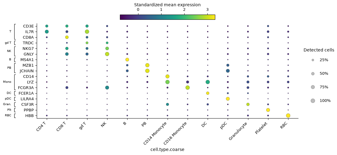
Before using the annotations, check them against well-known PBMC markers. CyteArc resolves gene symbols without regard to case and raises an error for missing or ambiguous names. This panel uses genes present in the published dataset.

The dot plot then reads only these genes from the remote counts. Values are library-size normalized counts (the assay default) with log1p; standardize="feature" rescales each gene so weakly and strongly expressed markers are equally visible. Dot size is the fraction of cells with nonzero expression.

# Group canonical PBMC markers by the identities they support.
marker_sets = {
    "T": ["CD3E", "IL7R", "CD8A"],
    "gd T": ["TRDC"],
    "NK": ["NKG7", "GNLY"],
    "B": ["MS4A1"],
    "PB": ["MZB1", "JCHAIN"],
    "Mono": ["CD14", "LYZ", "FCGR3A"],
    "DC": ["FCER1A"],
    "pDC": ["LILRA4"],
    "Gran.": ["CSF3R"],
    "Plt": ["PPBP"],
    "RBC": ["HBB"],
}

# Choose four interferon-response genes for the next comparison.
isg_genes = ["IFI27", "ISG15", "IFI44L", "IFI6"]

Started: 2026-10-12T13:57:20.528399Z | Wall time: 0.005 s

# Compare marker expression and detection across cell types.
ds.plots.dotplot(
    features=marker_sets,
    group_by="cell.type.coarse",
    group_order=coarse_order,
    normalization=NormalizationSpec(transform="log1p"),
    standardize="feature",
    figsize=(11, 5),
    max_figure_width=None,
)

$Marker dot plot across coarse blood-cell types. Dot color shows standardized mean expression and size shows detection fraction; expected lineage markers support the published annotations.$

Started: 2026-10-12T13:57:20.534093Z | Wall time: 16.669 s

Each population is brightest for its expected markers: TRDC in gamma-delta T cells, GNLY and NKG7 in NK cells, MS4A1 in B cells, MZB1 and JCHAIN in plasmablasts, CD14 and LYZ in CD14 monocytes, FCGR3A in CD16 monocytes, FCER1A in DCs, LILRA4 in pDCs, PPBP in platelets, and HBB in erythrocytes. Detection fractions are modest for some markers, including CD3E and CD14, so read dot size alongside its colour. This panel supports using the published labels for the comparisons below; it is a check of selected markers, not an independent annotation of every cell.

Interferon response¶

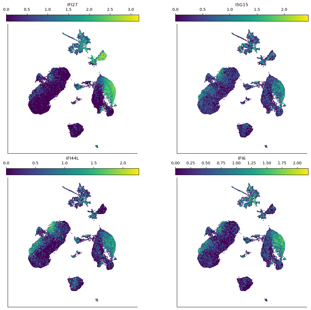
Type I interferon-stimulated genes (ISGs) are a common readout of antiviral signalling. This section looks at four: IFI27, ISG15, IFI44L, and IFI6. sort_values=True draws high-expressing cells on top.

# Plot the four interferon-response genes on the imported UMAP.
ds.plots.embedding(
    layout=umap_ref,
    color_by=isg_genes,
    normalization=NormalizationSpec(transform="log1p"),
    sort_values=True,
    n_columns=2,
    figsize=(11, 10),
)

Blood-cell UMAP panels show log-normalized IFI27, ISG15, IFI44L, and IFI6 expression. IFI27 is more restricted to parts of the monocyte and erythrocyte regions than the other three genes.

Started: 2026-10-12T13:57:37.204497Z | Wall time: 17.132 s

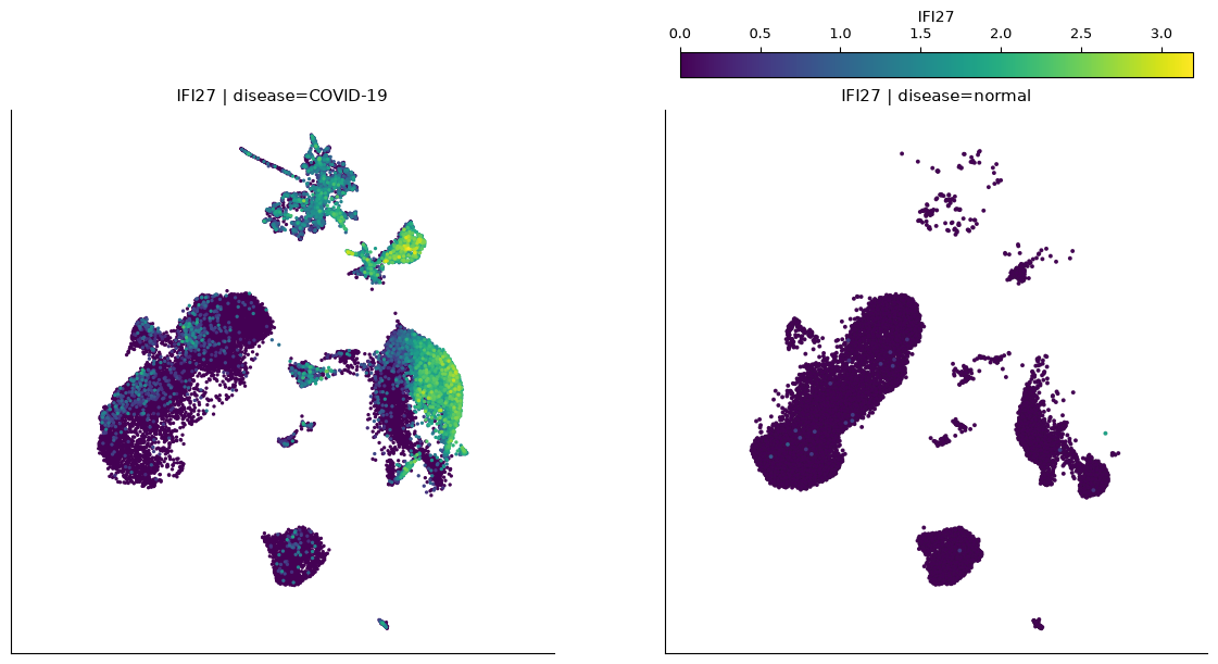
ISG15, IFI44L, and IFI6 are expressed across many cell types, with the highest values in the right half of the monocyte island and in parts of the T and NK area. IFI27 is more restricted: it is concentrated in that same monocyte region and in the erythrocyte cluster. Faceting IFI27 by condition, on a shared color scale, shows where the signal comes from:

# Compare IFI27 expression between conditions on a shared scale.
ds.plots.embedding(
    layout=umap_ref,
    color_by=isg_genes[0],
    facet_by="disease",
    normalization=NormalizationSpec(transform="log1p"),
    sort_values=True,
    figsize=(12, 6),
)

IFI27 expression on matching COVID-19 and healthy UMAP panels with a shared color scale. Strong signal occurs in COVID-19 monocytes and erythrocytes and is largely absent in healthy cells.

Started: 2026-10-12T13:57:54.337565Z | Wall time: 14.788 s

IFI27 is essentially absent from healthy cells. In COVID-19 samples it is strongest in the shifted monocytes noted in “The published UMAP” section and in the erythrocyte cluster.

Compare donors, not cells¶

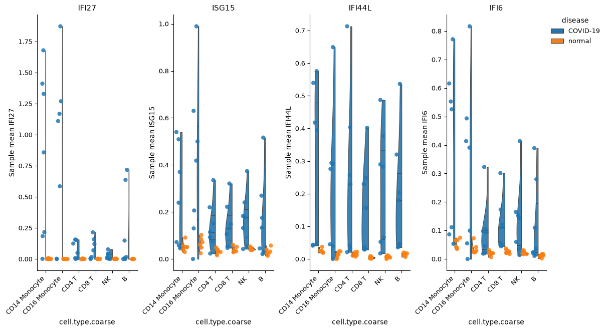
The cells come from only 13 people. Treating thousands of cells as independent biological replicates can overstate the evidence for a difference between conditions. Passing sample_by="donor_id" makes CyteArc average expression within each donor first, so each point below is one donor’s mean within a cell type; split_by="disease" puts the two conditions side by side.

# Focus the donor comparison on the major immune populations.
main_types = ["CD14 Monocyte", "CD16 Monocyte", "CD4 T", "CD8 T", "NK", "B"]

# Compare distributions within the stated groups.
ds.plots.distribution(
    isg_genes,
    grouping=CellField("cell.type.coarse"),
    groups=main_types,
    split_by="disease",
    sample_by="donor_id",
    normalization=NormalizationSpec(transform="log1p"),
    share_y=False,
    point_size=6,
    point_alpha=0.85,
    figsize=(12, 6.5),
    max_figure_width=None,
)

Donor-mean IFI27, ISG15, IFI44L, and IFI6 expression across six immune-cell types. Healthy donors remain near zero, while COVID-19 donors vary widely and some overlap the healthy range.

Started: 2026-10-12T13:58:09.126977Z | Wall time: 19.636 s

Healthy donors (orange) sit near zero for all four genes in every cell type. COVID-19 donors (blue) spread widely: several are far above the healthy range, while a few overlap it. The response is heterogeneous between patients.

To see which patients differ, summarize CD14 monocytes per donor in pandas. get_cell_vals returns one gene’s normalized values for the active cells selected by I. The code requests four genes without materializing the complete expression matrix; each request may fetch count blocks containing additional genes. ISG mean averages the four log1p values per cell. The last column is the authors’ per-cell IFN1 score averaged per donor; the original study defines it.

# Resolve the selected cells and four genes once for a single batched read.
cell_indices = ds.cells.active_index("I")
gene_indices = ds.RNA.feats.get_index_by(isg_genes, "names")

# Normalize the four genes together and log-transform their values.
expression = pd.DataFrame(
    np.log1p(ds.RNA.normed(cell_idx=cell_indices, feat_idx=gene_indices).compute()),
    index=meta.index,
    columns=isg_genes,
)

# Average the four log-transformed values within each cell.
expression["ISG mean"] = expression[isg_genes].mean(axis=1)

# Preview the four-gene expression table and per-cell mean.
expression.head()

	IFI27	ISG15	IFI44L	IFI6	ISG mean
ids
covid_555_1.1	1.960800	0.000000	0.0	0.0	0.490200
covid_555_1.2	0.000000	0.000000	0.0	0.0	0.000000
covid_555_1.3	1.765848	0.961459	0.0	0.0	0.681827
covid_555_1.7	0.000000	0.000000	0.0	0.0	0.000000
covid_555_1.8	0.926000	0.000000	0.0	0.0	0.231500

Started: 2026-10-12T13:58:28.765109Z | Wall time: 10.630 s

Restrict the summary to CD14 monocytes and compare donors.

# Keep CD14 monocytes and their aligned expression values.
monocytes = meta.join(expression).query("`cell.type.coarse` == 'CD14 Monocyte'")

# Average gene scores within each donor's monocytes.
mono_table = monocytes.groupby("donor_id").agg(
    disease=("disease", "first"),
    admission=("Admission", distinct),
    ventilated=("Ventilated", distinct),
    monocytes=("disease", "size"),
    **{column: (column, "mean") for column in [*isg_genes, "ISG mean", "IFN1"]},
)

# Inspect the expression and clinical summary for each donor's monocytes.
mono_table.round(3)

	disease	admission	ventilated	monocytes	IFI27	ISG15	IFI44L	IFI6	ISG mean	IFN1
donor_id
C1	COVID-19	ICU	NonVent / Vent	3419	1.329	0.370	0.395	0.553	0.662	0.149
C2	COVID-19	ICU	NonVent	217	0.216	0.046	0.049	0.111	0.105	0.042
C3	COVID-19	ICU	Vent	1102	0.184	0.072	0.044	0.086	0.096	0.040
C4	COVID-19	ICU	Vent	713	1.411	0.239	0.418	0.525	0.648	0.155
C5	COVID-19	ICU	NonVent	462	1.679	0.540	0.539	0.771	0.882	0.193
C6	COVID-19	ICU	Vent	277	0.858	0.509	0.575	0.616	0.640	0.183
C7	COVID-19	Floor	NonVent	2095	0.001	0.058	0.041	0.053	0.038	0.065
H1	normal	N/A	Healthy	680	0.000	0.030	0.025	0.035	0.022	0.039
H2	normal	N/A	Healthy	325	0.000	0.050	0.019	0.066	0.034	0.044
H3	normal	N/A	Healthy	215	0.000	0.039	0.020	0.042	0.025	0.045
H4	normal	N/A	Healthy	166	0.000	0.051	0.023	0.066	0.035	0.035
H5	normal	N/A	Healthy	444	0.001	0.091	0.037	0.075	0.051	0.055
H6	normal	N/A	Healthy	224	0.008	0.055	0.024	0.040	0.032	0.038

Started: 2026-10-12T13:58:39.397478Z | Wall time: 0.026 s

This table gives one expression summary per donor. As an optional numerical check, compare the seven patient means with the six healthy means and compare the four-gene summary with the authors’ IFN1 score. These are exploratory checks, not a model of disease severity.

# Select the patient donor means.
covid = mono_table.loc[mono_table["disease"] == "COVID-19", "ISG mean"]

# Select the healthy donor means.
healthy = mono_table.loc[mono_table["disease"] == "normal", "ISG mean"]

# Compare the independent donor means with a two-sided rank test.
test = mannwhitneyu(covid, healthy, alternative="two-sided")

# Compare the four-gene summary with the authors' interferon score.
rho = spearmanr(mono_table["ISG mean"], mono_table["IFN1"]).statistic

# Count patients above the highest healthy donor mean.
n_above = (covid > healthy.max()).sum()

# Show how many patient means exceed the highest healthy donor.
print(f"Patients above the highest healthy donor: {n_above} of {len(covid)}")

# Report the donor-level rank statistic and two-sided p-value.
print(
    f"Mann-Whitney U on donor means ({len(covid)} vs {len(healthy)} donors): "
    f"U = {test.statistic:.0f}, two-sided p = {test.pvalue:.4f}"
)

# Report concordance with the authors' interferon-response score.
print(
    "Spearman correlation of donor ISG mean with the authors' IFN1 score:",
    f"{rho:.2f}",
)

Patients above the highest healthy donor: 6 of 7
Mann-Whitney U on donor means (7 vs 6 donors): U = 41, two-sided p = 0.0023
Spearman correlation of donor ISG mean with the authors' IFN1 score: 0.73

Started: 2026-10-12T13:58:39.424851Z | Wall time: 0.009 s

In CD14 monocytes, six of the seven patients have a higher ISG mean than any healthy donor. C1, C4, C5, and C6 are highest (about 0.64 to 0.88, against at most 0.05 in healthy donors), C2 and C3 are modestly elevated, and C7, the one patient on a general ward rather than in intensive care, lies within the healthy range. The authors’ IFN1 score ranks donors in a similar order, so this four-gene summary agrees with the study’s own score. C1’s two samples (days 9 and 11) are pooled throughout because the summaries group by donor_id.

Takeaways¶

Working only from the remote store, with cell metadata and 21 genes:

Study design came from metadata: 7 COVID-19 patients and 6 healthy donors, so the donor is the unit for every comparison.
Composition: plasmablasts make up a larger fraction of recovered cells in every patient (C7 only marginally), while CD16 monocytes, gamma-delta T cells, pDCs, and NK cells make up smaller fractions in most patients.
Cell state: CD14 monocytes from COVID-19 samples occupy a distinct region of the published UMAP, the same region with the highest interferon-stimulated gene expression.
Interferon response: elevated in most but not all patients. Showing each donor’s mean makes the variation between patients visible.
Annotations: the published labels agree with canonical PBMC markers.

Limitations¶

These are descriptive observations on published annotations from one cohort. See the original study for its full analysis and clinical context.
The Mann-Whitney test compares 7 donor means with 6, so its p-value reflects 13 biological replicates rather than thousands of cells. Treat it as one exploratory test: the genes, cell type, and summary were chosen after looking at the data, and 13 donors cannot account for age, sex, sampling day, or treatment.
The read-only store cannot save results. For new embeddings, clustering, marker detection, or donor-level testing with compare.test, mount the dataset so new results are written locally while the counts stay in the bucket:

# Mount a writable analysis store while keeping counts remote.
analysis_ds = catalog.mount_datastore(entry.id, at="./analysis.zarr")

See Compare biological conditions across donors and Pseudobulk and differential expression (DE) primer for formal condition analyses, Explore a remote dataset for mounted analysis, and Explore CyteBase for catalog search and SQL queries.

References¶

Wilk, A. J., Rustagi, A., Zhao, N. Q., Roque, J., Martínez-Colón, G. J., McKechnie, J. L., Ivison, G. T., Ranganath, T., Vergara, R., Hollis, T., Simpson, L. J., Grant, P., Subramanian, A., Rogers, A. J., & Blish, C. A. (2020). A single-cell atlas of the peripheral immune response in patients with severe COVID-19. Nature Medicine, 26(7), 1070–1076. 10.1038/s41591-020-0944-y
Abdulla, S., Aevermann, B., Assis, P., Badajoz, S., Bell, S. M., Bezzi, E., Cakir, B., Chaffer, J., Chambers, S., Cherry, J. M., Chi, T., Chien, J., Dorman, L., Garcia-Nieto, P., Gloria, N., Hastie, M., Hegeman, D., Hilton, J., Huang, T., … Carr, A. (2024). CZ CELLxGENE Discover: a single-cell data platform for scalable exploration, analysis and modeling of aggregated data. Nucleic Acids Research, 53(D1), D886–D900. 10.1093/nar/gkae1142