Pseudotime orders cell states along a process. Fate mapping adds a different question: how strongly does each cell connect to several possible endpoints?
CyteArc models walks through the cell graph, favoring movement toward higher pseudotime. The chosen terminal populations act as absorbing endpoints: once a walk reaches one, it stops. The probability of reaching each endpoint summarizes the cell’s position relative to those choices. It does not track a living cell or prove its future identity.
We continue the developing-pancreas example from Order cell states with pseudotime, using Alpha, Beta, and Delta as candidate outcomes. Their familiar markers include Gcg, Ins1/Ins2, and Sst, respectively. Published annotations guide this example; another dataset needs its own endpoint evidence.
Open the prepared analysis
# Import array operations and CyteArc for defining trajectory endpoints.
import numpy as np
import pandas as pd

import cytearc
from cytearc.plotting import CellField, ColorScale

# Keep routine progress messages out of the teaching output.
cytearc.configure_output(level="WARNING", progress=False)

# Download the prepared example, including its saved analysis.
dataset = cytearc.cytebase.connect("cytearc_docs").download_dataset(
    name="bastidas-ponce_4K_pancreas-d15_rnaseq",
    destination="cytearc_datasets",
    zarr=True,
)
Started: 2026-10-11T18:54:47.893665Z | Wall time: 5.273 s
Open the downloaded store and its saved analysis.
# Open the datastore for the following analysis.
ds = cytearc.DataStore(f"{dataset}/data.zarr", nthreads=4)

# Reuse the saved run and its frozen cell selection.
analysis_run = ds.pipeline.open(label="docs_default")

# Keep the graph used by the saved analysis.
graph = analysis_run["connectivity_map"]

# Inspect the opened assays and their dimensions.
ds
DataStore has 3696 (3696) cells with 1 assays: RNA
Cell metadata:
'I', 'ids', 'names', 'G2M_score', 'RNA_UMAP1',
'RNA_UMAP2', 'RNA_clusters', 'RNA_leiden_cluster', 'RNA_nCounts', 'RNA_nFeatures',
'RNA_percentMito', 'RNA_percentRibo', 'S_score', 'clusters', 'clusters_coarse'
RNA assay has 27998 features and following metadata:
'I', 'ids', 'names', 'dropOuts', 'highly_variable_genes',
'nCells'Started: 2026-10-11T18:54:53.170743Z | Wall time: 3.857 s
Orient the graph
Repeat the source and sink weighting from Order cell states with pseudotime. Ductal cells share a total of -1, and all Alpha, Beta, and Delta cells together share +1. These totals balance the source against the pooled sinks; they do not give each terminal cell type equal weight.
# Read the published cell-type labels for the selected cells.
annotations = ds.cells.fetch("clusters", key="I")

# Mark ductal cells as the source population.
source = annotations == "Ductal"

# Mark the pooled terminal populations.
sink = np.isin(annotations, ["Alpha", "Beta", "Delta"])

# Require at least one annotated source cell and one sink cell.
if not source.any() or not sink.any():
    raise ValueError("Source and sink annotations must both be present")

# Start every graph cell with zero source or sink mass.
source_sink_vector = np.zeros(len(annotations), dtype=float)

# Share total mass -1 among the source cells.
source_sink_vector[source] = -1.0 / source.sum()

# Share total mass +1 among the pooled sink cells.
source_sink_vector[sink] = 1.0 / sink.sum()

# Orient the graph using the chosen source and sinks.
pseudotime_ref = ds.trajectory.pseudotime(graph, ss_vec=source_sink_vector)

# Check the number of cells used to orient the graph.
pd.Series({"source cells": int(source.sum()), "sink cells": int(sink.sum())})
source cells 916
sink cells 1142
dtype: int64Started: 2026-10-11T18:54:57.031062Z | Wall time: 0.641 s
Select the terminal populations
The live clusters column above contains published cell-type names. The saved run’s
clusters result contains computed integer labels. For this example we choose one
computed cluster per candidate fate, using its most common published annotation.
First inspect the annotation shares within each computed cluster. These two label arrays cover the same selected cells in the prepared store.
# Keep the computed clustering used to define terminal boundaries.
sink_labels_ref = analysis_run["clusters"]

# Read its labels in the run's cell order.
sink_labels = analysis_run.cells.fetch("clusters")

# Check that imported and computed labels cover the same cell count.
assert len(annotations) == len(sink_labels)

# Measure each published annotation's share within each cluster.
shares = pd.crosstab(
    sink_labels,
    annotations,
    rownames=["cluster"],
    colnames=["annotation"],
    normalize="index",
)

# Show the majority annotation and its share for every cluster.
sink_table = pd.DataFrame(
    {"annotation": shares.idxmax(axis=1), "majority share": shares.max(axis=1)}
)

# Inspect every candidate cluster before choosing terminal boundaries.
sink_table| annotation | majority share | |
|---|---|---|
| cluster | ||
| 1 | Pre-endocrine | 0.843915 |
| 2 | Ductal | 0.769231 |
| 3 | Alpha | 0.862069 |
| 4 | Ductal | 0.967442 |
| 5 | Ductal | 0.672646 |
| 6 | Pre-endocrine | 0.605882 |
| 7 | Epsilon | 0.658537 |
| 8 | Ductal | 0.827586 |
| 9 | Delta | 0.741935 |
| 10 | Beta | 0.984000 |
| 11 | Ngn3 high EP | 1.000000 |
| 12 | Ngn3 high EP | 0.699588 |
Started: 2026-10-11T18:54:57.674678Z | Wall time: 0.122 s
Keep the clusters whose majority annotations match our three candidate fates. Requiring one cluster per fate makes a missing or ambiguous choice visible instead of selecting an endpoint arbitrarily.
# Choose the three candidate terminal identities.
candidate_fates = ["Alpha", "Beta", "Delta"]

# Keep one cluster for each requested terminal identity.
selected = sink_table.loc[sink_table["annotation"].isin(candidate_fates)]

# Count the candidate fates before checking for missing or duplicated matches.
n_fates = len(candidate_fates)

# Check that each requested fate identifies exactly one cluster.
valid_fates = len(selected) == n_fates == selected["annotation"].nunique()

# Reject a missing or ambiguous terminal-cluster choice.
if not valid_fates:
    raise ValueError("Each candidate fate must match exactly one cluster")

# Keep the computed cluster label as a column.
selected = selected.reset_index(names="sink label")

# Index the table by the candidate annotation.
selected = selected.set_index("annotation")

# Match the order used for the probability columns and plots.
selected = selected.loc[candidate_fates]

# Extract the computed cluster labels for the terminal boundaries.
terminal_labels = selected["sink label"].astype(int).tolist()

# Attach readable fate names to those cluster labels.
sink_names = dict(zip(terminal_labels, candidate_fates, strict=True))

# Inspect the selected terminal clusters and their annotation purity.
selected| sink label | majority share | |
|---|---|---|
| annotation | ||
| Alpha | 3 | 0.862069 |
| Beta | 10 | 0.984000 |
| Delta | 9 | 0.741935 |
Started: 2026-10-11T18:54:57.799546Z | Wall time: 0.012 s
The selected Delta cluster has a majority share of about 0.74, so it includes cells with other annotations. Every cell in a selected cluster becomes a boundary for this model. This is an exploratory endpoint choice, not a pure set of terminal cells. Before using it for a biological claim, inspect marker evidence and compare alternative boundaries. See Annotate cell types and states for marker checks.
Calculate the probabilities
# Calculate absorption probabilities for the chosen endpoints.
fate_ref = ds.trajectory.fate(
    pseudotime_ref, sink_labels_ref, sinks=terminal_labels
)

# Load the probabilities and their validity mask.
fate = ds.trajectory.load_fate(fate_ref)

# Compare valid probability rows with the complete graph-cell count.
{"valid probability rows": int(fate.valid.sum()), "graph cells": len(fate.valid)}
{'valid probability rows': 3696, 'graph cells': 3696}Started: 2026-10-11T18:54:57.814126Z | Wall time: 2.634 s
The output reports how many graph cells have valid probabilities. Summarize only those rows. Each probability column is one candidate fate, and the columns should sum to one for each valid cell.
# Match fate names to the saved probability-column order.
fate_names = [sink_names[int(label)] for label in fate.sink_labels]

# Keep valid rows and label each probability column by fate.
probabilities = pd.DataFrame(fate.values[fate.valid], columns=fate_names)

# Measure each probability row's deviation from a total of one.
probabilities["row-sum error"] = abs(probabilities.sum(axis=1) - 1.0)

# Inspect probability ranges and the error in their row sums.
probabilities.agg(["min", "median", "max"])| Alpha | Beta | Delta | row-sum error | |
|---|---|---|---|---|
| min | 0.000000 | 0.000000 | 0.000000 | 0.000000e+00 |
| median | 0.345601 | 0.317223 | 0.308123 | 0.000000e+00 |
| max | 1.000000 | 1.000000 | 1.000000 | 1.192093e-07 |
Started: 2026-10-11T18:55:00.450914Z | Wall time: 0.016 s
A small row-sum error checks numerical consistency. Likewise, high probability at a chosen sink is imposed by the model. Neither check supplies independent evidence that the endpoint choice is biologically correct.
View the candidate outcomes
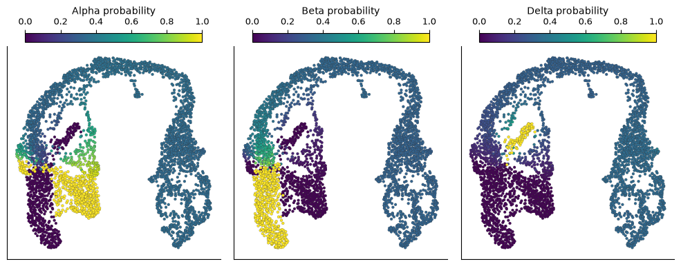
Store each probability as a cell column, then plot all three on the same zero-to-one color scale. This uses the same UMAP as the preceding trajectory analysis.
# Save each fate probability in the matching cell order.
for index, label in enumerate(fate.sink_labels):

    # Save the values in cell metadata using the stated selection.
    ds.cells.insert(
        f"fate_prob_{sink_names[int(label)]}",
        fate.values[:, index],
        key="I",
        overwrite=True,
    )

# Compare the three fate probabilities on a shared zero-to-one scale.
ds.plots.embedding(
    layout=analysis_run["umap"],
    color_by=[
        CellField(
            f"fate_prob_{name}", kind="continuous", label=f"{name} probability"
        )
        for name in candidate_fates
    ],
    n_columns=3,
    color_scale=ColorScale(scope="shared", vmin=0, vmax=1),
    sort_values=True,
)
Started: 2026-10-11T18:55:00.468941Z | Wall time: 1.962 s
Look for where the model favors one outcome and where it divides probability between outcomes. A mixed probability describes this graph and its endpoints; it does not show that a cell has been observed to choose between those fates.
Common mistakes and limitations
The candidate list is incomplete: the dataset also contains Epsilon cells, and valid cells must distribute their probability among the three selected outcomes, so this example cannot describe every endocrine fate.
Reading model structure as biology: smooth gradients can come from graph averaging across an abrupt transition, and the probabilities depend on the chosen endpoints and graph, so compare plausible alternatives with Trajectory validation checklist before making a firm lineage claim.
Invalid cells have no interpretable probabilities: check how many cells are invalid and which graph components they hold before drawing conclusions.
Use Follow gene expression along pseudotime to inspect gene profiles along the same pseudotime axis.