Pseudotime places cells along an ordering, but the ordering alone does not tell us what changes along the way. Some genes increase or decrease steadily from progenitor to terminal population. Others rise briefly and fall again. A correlation score can detect a steady trend while missing a transient peak with little overall rise or fall.
Expression dynamics makes these patterns easier to inspect: we smooth each gene’s expression along the ordering, then group genes with similar profiles into modules. A module might contain genes that fade early, turn on late, or peak in the middle. Here we use the pancreas analysis to build and interpret those modules.
Start with Order cell states with pseudotime for the endpoint choices and scoring method. This page uses the same ordering and focuses on how to read the expression heatmap.
Open the prepared analysis and orient its graph
# Load array and table tools alongside the analysis package.
import numpy as np
import pandas as pd

import cytearc

# Keep routine progress messages out of the teaching output.
cytearc.configure_output(level="WARNING", progress=False)

# Download the prepared example, including its saved analysis.
dataset = cytearc.cytebase.connect("cytearc_docs").download_dataset(
    name="bastidas-ponce_4K_pancreas-d15_rnaseq",
    destination="cytearc_datasets",
    zarr=True,
)
Started: 2026-10-11T18:54:47.052569Z | Wall time: 4.281 s
Open the downloaded store and its saved analysis.
# Open the datastore for the following analysis.
ds = cytearc.DataStore(f"{dataset}/data.zarr", nthreads=4)

# Reuse the saved run and its frozen cell selection.
analysis_run = ds.pipeline.open(label="docs_default")

# Keep the graph used by the saved analysis.
graph = analysis_run["connectivity_map"]

# Use the complete feature universe for this assay.
all_features = analysis_run["feature_universe"]

# Inspect the opened assays and their dimensions.
ds
DataStore has 3696 (3696) cells with 1 assays: RNA
Cell metadata:
'I', 'ids', 'names', 'G2M_score', 'RNA_UMAP1',
'RNA_UMAP2', 'RNA_clusters', 'RNA_leiden_cluster', 'RNA_nCounts', 'RNA_nFeatures',
'RNA_percentMito', 'RNA_percentRibo', 'S_score', 'clusters', 'clusters_coarse'
RNA assay has 27998 features and following metadata:
'I', 'ids', 'names', 'dropOuts', 'highly_variable_genes',
'nCells'Started: 2026-10-11T18:54:51.340575Z | Wall time: 5.973 s
Use the published cell-type annotations to orient the graph. As in the pseudotime example, the source and pooled sinks each receive a total mass of one, with opposite signs.
# Read the published cell-type labels for the selected cells.
annotations = ds.cells.fetch("clusters", key="I")

# Mark ductal cells as the source population.
source = annotations == "Ductal"

# Mark the pooled terminal populations.
sink = np.isin(annotations, ["Alpha", "Beta", "Delta"])

# Require at least one annotated source cell and one sink cell.
if not source.any() or not sink.any():
    raise ValueError("Source and sink annotations must both be present")

# Start every graph cell with zero source or sink mass.
source_sink_vector = np.zeros(len(annotations), dtype=float)

# Share total mass -1 among the source cells.
source_sink_vector[source] = -1.0 / source.sum()

# Share total mass +1 among the pooled sink cells.
source_sink_vector[sink] = 1.0 / sink.sum()

# Orient the graph using the chosen source and sinks.
pseudotime_ref = ds.trajectory.pseudotime(graph, ss_vec=source_sink_vector)

# Check how many cells anchor the two ends of the ordering.
pd.Series({"source cells": int(source.sum()), "sink cells": int(sink.sum())})
source cells 916
sink cells 1142
dtype: int64Started: 2026-10-11T18:54:57.316863Z | Wall time: 0.749 s
Group changing expression profiles
Start with the default aggregation settings. CyteArc orders cells with valid pseudotime scores, then smooths each retained gene over a rolling 200-cell window. This replaces individual, often sparse measurements with a local average along the ordering, making shared trends easier to see. The smoothed profiles are summarized in 50 ordered bins with approximately equal cell counts, then grouped into 10 modules. A bin can cover a narrow or broad range of pseudotime depending on where cells are concentrated. The bins are not equal intervals of pseudotime or elapsed time.
# Group genes with similar expression profiles along pseudotime.
modules_ref = ds.trajectory.aggregation(pseudotime_ref, features=all_features)

# Display the ordered expression profiles and their modules.
ds.plots.pseudotime_heatmap(aggregation=modules_ref)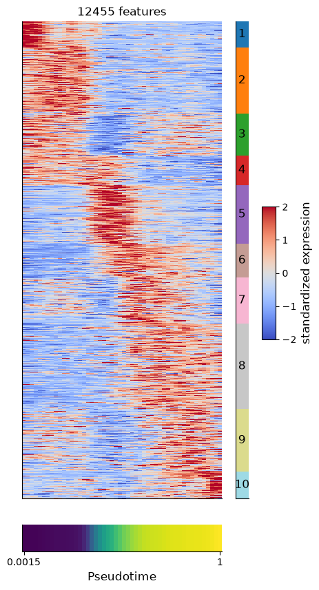
Started: 2026-10-11T18:54:58.068470Z | Wall time: 19.038 s
Read from early to late pseudotime across the heatmap. Look for groups that peak early, late, or in the middle. By default, each gene is scaled relative to its own variation. Red indicates higher expression and blue lower expression for that gene; the colours do not show which gene has the greatest absolute expression.
Module numbers are labels, not developmental stages. Ten modules is a starting choice, not a claim that the process has ten biological programs.
Inspect a module’s genes
Load the saved result to see how many genes each module contains:
# Load the saved gene-module assignments.
modules = ds.trajectory.load_aggregation(modules_ref)

# Pair each retained gene with its module label.
module_genes = pd.DataFrame({
    "gene": modules.feature_names,
    "module": modules.feature_clusters,
})

# Count the genes assigned to each expression module.
module_genes.groupby("module").size().rename("genes")
module
1 679
2 1732
3 1092
4 770
5 1537
6 871
7 1213
8 2231
9 1632
10 698
Name: genes, dtype: int64Started: 2026-10-11T18:55:17.108929Z | Wall time: 0.349 s
Choose a module from the heatmap, then list its genes. The example below selects the first module label only to show the lookup; the returned genes are not ranked markers.
# Choose the first module to demonstrate gene lookup.
module_id = module_genes["module"].min()

# Inspect the first twenty genes in the chosen module.
module_genes.loc[module_genes["module"] == module_id, "gene"].head(20)
17 Mcm3
26 Prim2
65 Stk17b
70 Hspd1
93 Bard1
137 Usp40
152 Pask
156 Dtymk
183 Zranb3
184 Mcm6
230 Dhx9
231 Npl
252 Klhl20
257 Fmo4
258 Fmo1
274 Nuf2
303 Fh1
319 Lbr
336 Cenpf
345 Dtl
Name: gene, dtype: strStarted: 2026-10-11T18:55:17.460670Z | Wall time: 0.007 s
Check whether several genes support a shared process before naming the module. Follow up candidate genes with marker maps or other independent evidence.
Adjust smoothing only when needed
A wide window can hide a brief expression peak; a narrow one can retain more noise. The width counts cells, not units of time. To explore a shorter window, repeat the call with one changed setting:
# Group genes with similar expression profiles along pseudotime.
modules_ref = ds.trajectory.aggregation(
    pseudotime_ref, features=all_features, window_size=100
)
n_clusters controls the requested number of modules and defaults to 10. chunk_size
controls the number of displayed pseudotime bins and defaults to 50; it is not a memory
batch size. Change one choice at a time and compare the profiles before interpreting
a split or merged module.
Common mistakes and limitations
Expression and variance checks exclude some features: genes with mean expression at or below
min_expor with no variation after smoothing are not retained, so the loaded result lists only the genes that passed those checks.Reading one axis as one path: pooling Alpha, Beta, and Delta into a shared sink can make lineage-specific genes look weak, and a shared ordering does not establish that all cells follow the same developmental route.
Over-reading the heatmap: per-gene scaling means the colours show relative change, not absolute abundance, and similar smoothed profiles need not share an upstream regulator or imply a causal role. Compare plausible endpoint and smoothing choices before treating a module as stable.
See Trajectory validation checklist for checks on orientation, valid cells, and endpoint sensitivity. Explore candidate cell fates describes several candidate terminal outcomes for each cell instead of assigning one position along an axis.